2016 International Conference on Mathematical, Computational and Statistical Sciences and Engineering (MCSSE 2016) ISBN: 978-1-60595-396-0
A Plant Recognition Method Based on Local Linear
Embedding and Multi-Feature Fusion
Zhang YANG, Bo FU
*, Ji-yuan LIU, Man-man MAO and Chen-xi OUYANG
School of Electrical & Electronic Engineering, Hubei University of Technology, Wuhan 430068, China
*Corresponding author
Keywords: Plant recognition, Local binary pattern, Local linear embedding, Shape features.
Abstract. In order to acquire the accurate and practical feature of leaves to improve the accuracy of leaves image recognition, a new method based on local linear embedding and multi-feature fusion is proposed. Firstly, the LBP algorithm is used to extract texture features of leaves. Considering the high dimension of LBP feature, local Linear embedding (LLE) algorithm is used to reduce the dimensions of leaf texture features. At the same time, the shape features of the leaves are considered. The LBP rotation invariant features are combined with the shape features. Then using the K nearest neighbor (KNN) method to recognize plant leaves. Experimental results based on the leaf image database prove that the proposed method has high recognition accuracy and stability.
Introduction
Plant recognition is a hot research topic in the current research of plant information science.[1] The early researchers usually use the features of leaf shape to do plant recognition. Ingronille and Arid [2] extracted 27 features of leaf shape, and then classify the oak tree with the method of principal component analysis; in 2001, Osikar et al.[3] extracted the features of geometric and moment of leaves, and classified 15 kinds of plants in Sweden by the feedforward neural network. Even though these methods have a higher rate of recognition when the sample is less, the rate of recognition would decline significantly when the methods are applied on recognize the plants with similar shape. Furthermore, the texture features of Gabor filter, gray level co-occurrence matrix and fractal dimension are also applied on leaves recognition, such as Cope et al.[4] extracted Gabor texture features of leaves to recognize more than 32 kind of plants. However, as the texture features are too simple, the recognition rate is not very ideal. In recent years, researchers combine the features of leaf shape and the texture features together to get higher recognition rate. For instance, Ding et al.[5] combined the features of leaf shape and leaf texture, and at the same time, they reduced the feature dimension by locally linear embedding (LLE) algorithm which improved the recognition precision and calculation efficiency of leaves effectively. But this method cannot be applied on the recognition problem when leaf rotation; Liu et al.[6] combined the texture features of LBP, gray level co-occurrence matrix, Gabor filter and the contour features of Hu invariant moment, Fourier operator together, and then used the deep belief network as the classifier structure to improve the recognition rate of leaf. However, this method takes a long time to do character calculation and training, so it has a negative effect on the recognition efficiency of algorithm.
This paper will combine the LBP texture features after LLE dimension reduction and the features of leaf shape together, and use K neighbor method to classify the images of plant leaf for recognition. The result shows that the combination of LBP texture features and leaf shape features contributes to improve the recognition results of plant leaf and computation efficiency.
The Texture Features of Leaf
35 10 140
50
12
32 55
17 81
1 0 1
1
0
1
0 1
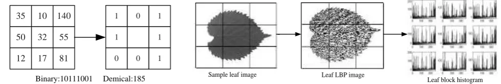
Binary:10111001 Demical:185 Sample leaf image Leaf LBP image Leaf block histogram
the recognition effect. LBP [7] algorithm is one of the effective texture extraction algorithm which is easy to calculate and the texture features is rich. In recent years, they are widely used in face recognition and other fields with a good effect.
LBP Operator
[image:2.595.51.541.234.316.2]Define a pixel window, and then compare the value of center pixel and surrounding pixel, if the value of surrounding pixel is bigger than the value of center pixels, the assignment of the value is 1; otherwise the assignment of the value is 0. In this way, it will produce an 8-bit unsigned binary number in eight points of neighborhood. According to the sum of different location and different weighting, it would produce a decimal number which is called LBP value of this window. Usually, this number is used to describe the texture information of the window, as shown in Figure 1.
Figure 1. Basic LBP operator. Figure 2. Image block and block histogram.
Using mathematical expression can be expressed as:
*2 1, 8 1
i i i c p s p pLBP
c
0 , 0 0 , 1 x x x s (1) Among them, i means there are eight pixel points around window, pi means the value of
surrounding pixel, pc means the value of center pixel,
c p
LBP means the LBP value after calculation.
From the LBP encoding process, when the position between the pixel changeless, and drab gray value changes, the encoding binary and the value of LBP will not change. So it proves that LBP is invariable to the change of drab gray or the change of light.
The LBP Features of Leaf
In order to extract the texture features of leaf, the LBP algorithm references to the image of leaf. Equal the image of leaf on the horizontal axis and the vertical axis [8] to get more sufficient information, the general block is 3*3, 4*4 and 5*5 et al., LBP was calculated on each block, and then use histogram to statistic model number, then get the histogram vector, as shown in figure 2.
Dividing the leaf image into M pieces, then encoding each image with LBP code respectively. Set LBP (xj, yj) as the LBP feature images after calculating the original image. Use j as the block of image, j=1,2,...,M. Each sub-block histogram vector as follow:
j j y x j ji T LBP x y i
R , } ) , ( { (2) Among them, use i as the level of gray, i=0, 1, 2,...,255. In the region M, R stands for the number of pixel in the i gray value. When a = true, T(a) = 1; when a = false, T(a) = 0.
In order to get a combination of histogram vector connected every histogram vector together.
} ) ( , ) ( , )
{(Ri 1 Ri 2 Ri M
H , (3)
Locally Linear Embedding Algorithm
After equal the image of leaf, the dimension of the LBP histogram vector of leaf image has risen sharply, which affected to the speed of algorithm seriously. In order to solve the problem of the excessive LBP feature dimension, using the local linear embedding (LLE) algorithm [9] to reduce dimension of the histogram vector.
Assumes a high-dimensional database X
x1,x2, ,xn
RD, the specific steps of LLE algorithmis: calculating all the Euclidean distance between the sample points in the database X , and then try to find K sample points which are close to sample point xi in Euclidean distance, all these sample points
consist of K neighborhood for xi.
Using the point which near the sample point xi and its weight Wij to represent xi in linear, and then calculating the local reconstruction matrix W of the sample point xi to make the minimum error
of the reconstruction function
W ;Among them,
21
i
K
j j ij i W x
x W
(4) A weigh matrix W is consist of Wij. So it must meet two conditions. Firstly, when xj is not belong
to the neighborhood of xi, Wij 0;otherwise, 1 1
k
j ij
W . Calculating space mapping yi of the
sample point xi in low-dimensional, minimize the weighted error of i
W function; In which,
T ji ij
ij n
i
j ij i
i W
y
W y
M y y 2
1
(5) And from (12),
I W
I W
M T (6)
Do the sparse diagonalization to sparse symmetric matrix M, can get (d+1) smaller eigenvectors corresponding eigenvalues. Mapping the sample collection X to a low-dimensional space, the output of the low-dimensional Y is the eigenvectors from 2 to (d+1) corresponding eigenvalues of matrix M.
LLE algorithm is able to reduce feature dimension under the condition of retain the main texture feature information, and reduce the amount of calculation also. At the same time, LLE could introduce the category information of the sample leaf image into algorithm. It reduces the distance between same class, and increases the distance between different class, so the samples are easy to recognize.
The Features of Leaf Shape
The leaf shape is different between different kinds of plant leaves. So the features of leaf shape include lots of important information about the plant classification. In this issue, the authors extracted 7 features of leaf shape as auxiliary features associated with LBP features to recognize plant species.
The Geometry Parameters of Leaf
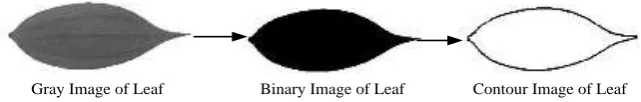
Gray Image of Leaf Binary Image of Leaf Contour Image of Leaf
Figure 3. Leaf contour extraction process.
(1) Perimeter: The total length of leaf Lleaf.
(2) Area: Indicating the total pixel number inside the leaf Sleaf.
(3) Long axis: The farthest distance between two pixels on the leaf profile llong_axis.
(4) Minor axis: Vertical to the long axis,the nearest distance between two pixels on the leaf profile lminor_axis.
(5) Convex hull area: Indicating a minimum convex hull area which can cover all the pixels of leaf
hull convex
S _ .
(6) Convex hull Perimeter: The total length of the convex hull profile Lconvex_hull.
Describe the Geometric Features of Leaf
Through the above geometric parameters, seven geometric description features can be calculated. (1) The ratio of vertical and horizontal axis: the ratio of vertical and horizontal axis about the external rectangular of leaf, that is:
Aspect ratio= Externalrectangle rectangle External
b a
(7) (2) The rectangle degree: The ratio of the area of leaf and the external rectangle area, that is:
The rectangle degree= Externalrectangle Externalrectangle leaf
b a
S
(8) (3) The ratio of concave area and convex area: The ratio of the convex hull area and the leaf area, that is:
Aconvexity = convex_hull leaf
s s
(9) (4) The ratio of concave and convex for perimeter: The ratio of the leaf profile length and the total length of convex hull, that is:
Pconvexity = convex_hull leaf
L L
(10) (5) The ratio of eccentricity: The ratio of long axis and short axis for leaf, that is:
Eccentricity= minor_axis axis _ long
l l
(11) (6) The shape parameter: The ratio of leaf area square value and leaf perimeter square value, that is:
The shape parameter= 2leaf leaf
L S 4
0.7 0.75 0.8 0.85 0.9 0.95
30 35 40 45 50
R
ecognition
R
ate
Sample Space
LBP
Gray level co- occurrence matrix + fractal dimension + shape LBP+shape
(7) The ratio of the perimeter and diameter: The ratio of the leaf perimeter and the main pulse length, that is:
Perimeter ratio of diameter = long_axis leaf
l L
(13) Though all these ratio calculations above, belongs to the relative features of shape, therefore in the rotation or scaling of leaf image, it keeps invariance.
The Experiment and Analysis
In order to verify the recognition result of leaf image by LBP, in this paper, collected about 50 kinds of common plant in the life for experiment. All the experiment images come from botanical garden of Wuhan, as shown in figure 4. Firstly, gray all the images and normalize their size to 320*240. Then, make a training set consist of leaf images from different directions. The training set has 15 images. Select from 50 kinds of plants as test targets randomly. And then, equal image into 3*3 blocks and extract its LBP features. Every image could extract 3*3*256=2304 dimensions of LBP features. Lastly, use LLE to reduce the dimensions into 50, extract 7 dimension of the shape feature from leaf, 16 dimensions of gray level co-occurrence matrix and 1 dimension texture dimension of fractal dimension. Use k neighbor method to recognize features to get recognition rate.
Figure 4. Gray images of some leaves. Figure 5. The recognition rate of three methods.
Experiment is under Windows 7 environment, the processor is the second generation of Intel core [email protected], the memory size is 4G. Compare the three experiment methods above by MATLAB (2013a) software. At the same time, use different number of sample space to get a comprehensive result. The experiment is under 30, 35, 40, 45, 50 sample space, respectively. Here comes the result.
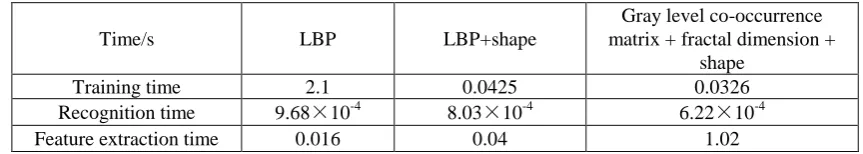
Table 1. The compare table about calculation time.
Time/s LBP LBP+shape
Gray level co-occurrence matrix + fractal dimension +
shape
Training time 2.1 0.0425 0.0326
Recognition time 9.68×10⁻⁴ 8.03×10⁻⁴ 6.22×10⁻⁴
Feature extraction time 0.016 0.04 1.02
In order to compare the calculation time of three methods, calculate the training time, recognition time and extract a leaf feature time of each method respectively. As shown in Table 1, because of large dimension of the original LBP algorithm, so it takes a longer time in training than the other two methods; All the recognition time of these methods are less than 1ms which can satisfy the need of practical application; when extract a image feature, the gray co-occurrence matrix method and the fractal dimension combined with shape feature method takes a long time about 1.02s, but the other two methods take a shorter time. Therefore, LBP combined with leaf shape features not only can have a higher recognition, but also can have an efficient calculation time.
Conclusion
In order to improve the recognition rate, this paper proposes a LBP texture feature combined with leaf shape feature, calculate LBP high-dimensional feature of the leaf rich texture information, use LLE to reduce its dimension and then combine LBP reduced dimension with leaf shape feature. Use k neighbor method to recognize leaf. The experiment result indicate that, in the sample space of this paper, combine LBP feature with leaf shape feature can improve the accuracy of plant recognition effectively, and the calculation time is shorter, meanwhile the recognition time and calculation time is better than gray level co-occurrence matrix and fractal dimension combine with leaf shape feature. So it has a higher value of usage.
References
[1] Zhang N, Liu W P. Plant leaf recognition technology based on image analysis[J]. Application Research of Computers, 2011, 28(11):4001-4007.
[2] Ingrouille M J, Laird S M. A quantitative approach to oak- variability in some North London woodlands [J]. London Naturalist, 1986,65:34-46.
[3] Osikar J O. Computer vision classification of leaves from Swedish trees [D]. Linkoping: Linkoping University, 2001.
[4] Cope J S, Remagnino P, Barman S, et al. Plant Texture Classification Using Gabor Co-occurrences[C]//International Conference on Advances in Visual Computing. Las Vegas: Springer-Verlag, 2010:669-677.
[5] Ding J, Liang D, Yan Q. Recognition method of multi-feature plant leaves based on D-LLE algorithm[J]. Computer Engineering & Applications, 2015.
[6] Liu N, Kan J M, Technology S O, et al. Plant leaf identification based on the multi-feature fusion and deep belief networks method[J]. Journal of Beijing Forestry University, 2016.
[7] Ojala T, Harwood I. A Comparative Study of Texture Measures with Classification Based on Feature Distributions[J]. Pattern Recognition, 1996, 29(1):51-59.
[8] Xian W, Yan Z, Xin M U, et al. The Face Recognition Algorithm Based on Improved LBP[J]. Opto-Electronic Engineering, 2012, 1(4):76-80.