Robust three dimensional best path phase unwrapping algorithm that avoids singularity loops

Robust three-dimensional best-path

phase-unwrapping algorithm that

avoids singularity loops

Hussein Abdul-Rahman,

_{Miguel Arevalillo-Herráez,}

_{Munther Gdeisat,}

_*

David Burton,

_{Michael Lalor,}

_{Francis Lilley,}

_{Christopher Moore,}

Daniel Sheltraw,

_{and Mohammed Qudeisat}

1_{Mobile Machine and Vision Lab (MMVL), Sheffield Hallam University, Faculty of ACES, Showcase 4114,}

Pond Street, Sheffield S1 1WB, United Kingdom

2

Department of Computing, University of Valencia, Avenida Vicente Andrés Estellés s/n, 46100 Burjassot, Valencia, Spain

3_{General Engineering Research Institute (GERI), Liverpool John Moores University, James Parsons}

Building Room 114, Byrom Street, Liverpool L3 3AF, United Kingdom

4

North Western Medical Physics Department, Christie Hospital, Wilmslow Road, Manchester, M20 4BX, United Kingdom

5_{Brain Imaging Center, Helen Wills Neuroscience Institute, University of California, Berkeley,}

3210F Tolman Hall, MC 3192, Berkeley, California 94720-3192, USA

*Corresponding author: [email protected]

Received 22 April 2009; revised 3 July 2009; accepted 10 July 2009; posted 15 July 2009 (Doc. ID 110452); published 4 August 2009

In this paper we propose a novel hybrid three-dimensional phase-unwrapping algorithm, which we refer to here as the three-dimensional best-path avoiding singularity loops (3DBPASL) algorithm. This algorithm combines the advantages and avoids the drawbacks of two well-known 3D phase-unwrapping algorithms, namely, the 3D phase-unwrapping noise-immune technique and the 3D phase-unwrapping best-path technique. The hybrid technique presented here is more robust than its predecessors since it not only follows a discrete unwrapping path depending on a 3D quality map, but it also avoids any singularity loops that may occur in the unwrapping path. Simulation and experimental results have shown that the proposed algorithm outperforms its parent techniques in terms of reliability and robustness. © 2009 Optical Society of America

OCIS codes: 100.2650, 120.5050, 100.5070.

1. Introduction

Phase unwrapping has applications in many ad-vanced imaging technologies where the required data are encoded in the form of a phase distribution, such as optical interferometry, synthetic aperture

radar (SAR), and magnetic resonance imaging (MRI). In many cases, the extracted phase consists of a range of values in the interval [−π,þπ]. This fact is usually a direct result of using the mathematical arctangent function or certain other trigonometric operations. A phase-unwrapping algorithm is then required to remove these phase discontinuities and recover the original continuous phase signal. In gen-eral, these phase jumps are resolved by either adding

or subtracting an integer multiple of 2π to each phase value.

During the past three decades, numerous tech-niques have been proposed to solve the phase-unwrapping problem [1]. These can generally be classified into four major categories: global error-minimization methods [2,3], residue-balancing meth-ods [4,5], quality-guided algorithms [6–8], and the use of calculated phase wrap regions [9]. A thorough re-view of the two-dimensional phase-unwrapping pro-blem has been presented in a book by Ghiglia and Pritt [1].

The group of global error-minimization algorithms formulate the phase-unwrapping process in terms of the minimization of a global function. All the algo-rithms in this class are known to be robust, but they are also computationally intensive. TheLp-norm and least-squares algorithms are typical examples from this category [2,3].

Residue-balancing algorithms search for residues in a wrapped phase map and attempt to balance po-sitive and negative residues by placing cut lines be-tween them. The role of these cut lines is to create an unwrapping barrier and prevent the unwrapping path from going through them. The placement of a particular set of cut lines for any given wrapped phase map is not unique, and they may be placed in many different arrangements and orientations. These algorithms are generally fast but they are not very robust [4,5].

Quality-guided algorithms depend on some form of measure of the quality of the raw wrapped phase data to guide the phase-unwrapping path. The main idea of these algorithms is to phase unwrap the high-est quality pixels first and the lowhigh-est quality pixels last, thereby preventing error propagation during the unwrapping process [6,7]. To this end, a quality map needs to be defined. The success or failure of these algorithms is strongly dependent on this qual-ity map. Many two-dimensional qualqual-ity-guided algo-rithms have been proposed during the past two decades and most of these algorithms tend to follow a continuous path while they unwrap the phase map. These are generally computationally efficient and their robustness varies from one algorithm to an-other. One quality-guided algorithm that tends to un-wrap the phase map following a discrete path was proposed in [8]. This fast algorithm was used to con-struct a robust fringe pattern analysis system for human body shape measurement [10].

Many applications produce three-dimensional (3D) wrapped phase volumes, such as the noncontact measurement of dynamic objects, multitemporal SAR interferometric measurements [11], 3D Fourier fringe analysis [12], and MRI [13]. A 3D phase vo-lume consists of an array of voxels [a single element in the 3D volume that is analogous to a pixel in two-dimensional (2D) terms] and may be visualized as a number of consecutive 2D wrapped phase maps. Although a 2D unwrapping algorithm could be used to unwrap each of these maps independently [14], 3D

phase-unwrapping techniques can potentially yield more reliable results by embedding the third dimen-sion into the unwrapping process.

Three-dimensional phase unwrapping is a tively new concept, and therefore at this time

rela-tively few 3D algorithms have so far been

proposed. In a similar manner to the groupings used for categorization of the 2D phase-unwrapping algo-rithms, these 3D techniques can be classified into residue-balancing, quality-guided, or global error-minimization techniques. In 2001, Huntley proposed a 3D noise-immune phase-unwrapping algorithm that extended the 2D residue-balancing method into three dimensions [15]. In this method, all residues in the phase volume are identified and these are then connected together to form singularity loops. These loops are then regarded as prohibited 3D barrier sur-faces through which the phase-unwrapping path must not cross during the phase-unwrapping pro-cess. This process is performed in a 3D manner that is analogous to the use of cut lines when phase un-wrapping is carried out in 2D form. Huntley shows that there is only a single solution to the formation of these singularity loops, which means that a unique solution does exist. This is in contrast to the case for 2D phase-unwrapping algorithms, where no un-ique solution necessarily exists.

Cusack and Papadakis proposed a robust 3D phase-unwrapping algorithm that was used to un-wrap MRI data [13]. This algorithm uses a quality measurement to guide the final unwrapping path. At each iteration, only those voxels whose quality exceeds a certain threshold are unwrapped. The un-wrapping of the remaining voxels is left to subse-quent iterations, during which the threshold value is gradually reduced until the entire unwrapping process is complete. A major problem with this algo-rithm is the large number of iterations that are re-quired to unwrap the entire phase volume, thereby adversely impacting execution time.

Jenkinson has proposed the phase region expand-ing labeller for unwrappexpand-ing discrete estimates (PRELUDE) 3D phase-unwrapping algorithm follow-ing a global error-minimization approach. This tech-nique divides the wrapped phase volume into multiple regions. These regions are chosen in such a way that each region contains no phase wraps, i.e., the regions meet at and border the phase wraps, but each 3D region so produced must not contain a wrap. The individual regions are treated as single units by the algorithm. The differences between the phase values at the interface of adjacent regions is then considered and a cost function is applied and then minimized. When the cost between two regions is at a minimum, the two regions merge together. The process continues until a single large region is left. Although this method has been designed to process 2D and 3D MRI data, it can easily be extended to per-mit the unwrapping ofN-dimensional data [16].

volume is unwrapped, guided by a quality measure and following a discrete unwrapping path [17–19]. The best-path algorithm unwraps the highest quality voxels first and the lowest quality voxels last to prevent error propagation. A brief overview of this algorithm is presented in Section2.

In this paper we propose a hybrid phase-unwrapping algorithm, which is referred to as the 3D best-path avoiding singularity loops (3DBPASL) algorithm. The 3DBPASL algorithm combines the 3D noise-immune algorithm proposed by Huntley in [15,20] with our own 3D best-path algorithm pro-posed in [17–19]. This results in a hybrid 3D phase-unwrapping technique that is more effective than its predecessors.

In Section2, the 3D best-path phase-unwrapping algorithm is briefly reviewed. Section3explains the motivation behind the proposed 3DBPASL algo-rithm. The technique is then presented in detail in Section 4. Section5 shows the results produced by the proposed method and compares them with those obtained using other world-leading 3D phase-unwrapping algorithms. Finally, some conclusions are drawn in Section 6.

2. 3D Best-Path Algorithm: a Brief Review

Since the proposed algorithm follows the same un-wrapping path as the 3DBP algorithm, it is perhaps worth briefly describing here how this unwrapping path is defined. For further details, the reader is ad-vised to refer to [19].

The 3DBP algorithm defines the unwrapping path via the following steps:

1. Determine the quality of all voxels.

2. Calculate the horizontal, vertical, and normal edge qualities—where an edge can be defined as the connection between two adjacent voxels. Set the quality of any edges that are connected to the image borders to zero so that they are processed last.

3. Sort the edges in descending order of quality. 4. Unwrap voxels in the order of descending edge quality, so that the voxels which form the highest quality edges are unwrapped first, according to the following rules:

A. If both voxels in the edge do not belong to any group and have not been unwrapped before, then the voxels are unwrapped with respect to each other and gathered into a single group.

B. If one of the voxels has been processed before and belongs to a group, but the other has not, then the voxel that has not been processed before is un-wrapped with respect to the other voxels in the group and then joins this group.

C. If both voxels have been processed before and both belong to different groups, then the smaller group is unwrapped with respect to the larger group. After that the two groups are joined together to con-struct a single group.

3. 3DBPASL Algorithm: the Main Advantages

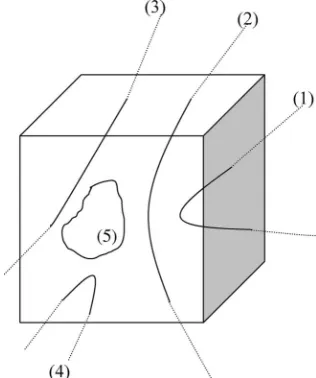
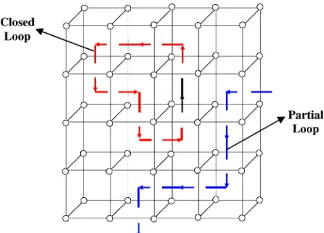
In three dimensions, phase singularities are shown to form loops in space, i.e., they appear connected so that they form either a closed loop or a partial loop that terminates at the boundary of the phase volume (see Fig.1). The 3D noise-immune phase-unwrapping algorithm works by placing branch-cut surfaces so as to prevent unwrapping through the phase singularity loops [15]. Then, unwrapping proceeds along any path that does not penetrate the surfaces (any such path would produce the same results, except for a constant multiple of2π). Unfortunately, the surfaces defined by the loops are not unique and there are several factors that may yield an incorrect result. One such factor is partial loops that begin and/or end at one side of the volume. Another problem is loop ambiguity.

Partial loops can be classified into three types:

• Partial loops that enter the wrapped phase vo-lume at one side of the vovo-lume and leave the vovo-lume from the same side. For example, partial loops 1 and 4 shown in Fig. 1.

• Partial loops that enter the phase volume at a side and leave from an adjacent side. For instance, the partial loop designated with the number 3 in Fig. 1.

• Partial loops that enter the phase volume at

one side and leave from the opposite side, such as the loop designated with the number 2 in Fig.1. In this paper, we refer to the last type as crossing loops.

Although the first two types of partial loop may also cause an incorrect unwrapping result, the latest type is specially relevant in the case of 3D measure-ment of dynamic objects. If the two ends of such a loop are joined with artificial residues as in [15], the branch-cut surface generated usually yields a discon-tinuity in each frame of the final result in the form of a straight line that joins a residue to the edge of the frame.

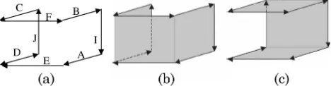
To explain the loop ambiguity problem, suppose that we have a wrapped phase volume consisting of

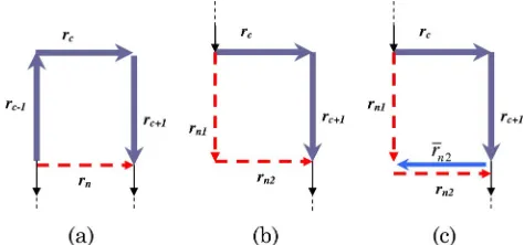
3×3×3 voxels. All the voxels in this volume have zero values except four as shown in Fig.2. The dots represent voxel points with values labeled near them as fractions of a cycle ofπ. This arrangement gener-ates three phase breaks, which have been indicated by red arrows. The purpose of establishing a phase singularity loop and its cut surface is to prevent any of the three phase breaks from being unwrapped. Clearly, there are residues associated with loops A, B, C, D, E, F, I, and J, but to draw a loop through them requires defining their polarity, since it is generally accepted that a positive residue should be connected only to a negative one and vice versa. A residue is considered positive if a positive phase discontinuity greater thanπis encountered in a counterclockwise loop around four pixels and it is considered negative if a negative phase discontinuity is encountered. What has to be considered for a three-dimensional set of voxels is on which side of the loop the observ-er is located. Given this convention, a loop connect-ing the residues in the figure presented above runs through the sequence of loops, B, F, C, J, D, E, A, I, and B as shown in Fig.3(a).

The problem with the loop is deciding what surface should be associated with it, and that is where the ambiguity arises. The two possible surfaces that could be constructed are shown in Figs.3(b)and3(c). The natural inclination is to use the smallest possi-ble surface, but here there are two possipossi-ble surfaces of equal size. One surface cuts through the three phase breaks shown in Fig. 3(b), and thus it will prevent their unwrapping, but the other, shown in Fig. 3(c), does not.

These ambiguities arise when some loops can be covered by two or more different surfaces; one of them is correct, whereas the others are incorrect. Obviously, if an incorrect surface is chosen, then bad data regions are still left unmarked and it is still possible for the unwrapping path to pass through this erroneous phase data. Hence, in this manner er-rors may propagate during the phase-unwrapping

process. Singularity loop ambiguities are discussed in detail by Salfity et al. in [21]. Therefore, it may be concluded that by relying solely upon locating and avoiding singularity loops, this approach may still lead to unexpected errors due to the potential for singularity loop ambiguity.

On the other hand, the best-path

phase-unwrapping algorithm does not identify singularity loops at all. Instead, it relies upon a quality measure to unwrap the phase volume. Ignoring singularity loops may cause the unwrapping path to penetrate these loops, and errors may propagate in the un-wrapped phase map.

The 3DBPASL algorithm proposed here takes ad-vantage of the unwrapping mechanisms of both of the former techniques to prevent error propagation. Initially, the proposed method identifies singularity loops and prohibits the unwrapping path from passing through them. It then ensures that the high-est quality voxels are unwrapped first and the worst quality voxels last. By integrating both mechanisms into the same hybrid algorithm, greater robustness is achieved.

4. 3DBPASL: the Algorithm

Here we present the 3DBPASL phase-unwrapping algorithm in detail. The key difference between this algorithm and the best-path algorithm is the intro-duction of the concept of zero-weighted edges, which are defined as edges that pass through a singularity loop, as shown in Fig.4.

The 3DBPASL algorithm can be outlined as follows:

1. Identify singularity loops.

2. Close all partial loops except crossing loops. 3. Identify zero-weighted edges.

4. Calculate all edge qualities and set the quality of all zero-weighted edges to zero.

Fig. 2. (Color online) Example of loops ambiguity in a3×3×3

wrapped phase volume.

Fig. 3. Singularity loop ambiguity resulting from a C-shaped loop.

5. Sort the edges according to their qualities: highest quality first, then in order of descending quality.

6. Unwrap the phase volume according to the

rules of the best-path phase-unwrapping algorithm described in the Section3.

These steps are explained in detail in the following subsections.

A. Identifying Singularity Loops

Residues in 3D volumes can be identified by calculat-ing phase differences in2×2loops located in thexy, xz, and yz planes. Identifying r_x residues requires calculating the phase difference in a loop located in the yz plane, while r_y residues are located in the zx plane and r_z residues are located in the xy plane, respectively [15,20].

Identifying r_x, r_y, and r_z residues is carried out using the following equations:

rx¼ℜ

_ψ

i;j;k−ψi;jþ1;k

2π

þℜ

_ψ

i;jþ1;k−ψi;jþ1;kþ1 2π

þℜ

_ψ

i;jþ1;kþ1−ψi;j;kþ1 2π

þℜ

_ψ

i;j;kþ1−ψi;j;k

2π

;

ð1Þ

ry¼ℜ

_ψ

i;j;k−ψi;j;kþ1 2π

þℜ

_ψ

i;j;kþ1−ψiþ1;j;kþ1 2π

þℜ

_ψ

iþ1;j;kþ1−ψiþ1;j;k

2π

þℜ

_ψ

iþ1;j;k−ψi;j;k

2π

;

ð2Þ

rz¼ℜ

_ψ

i;j;k−ψiþ1;j;k

2π

þℜ

_ψ

iþ1;j;k−ψiþ1;jþ1;k

2π

þℜ

_ψ

iþ1;jþ1;k−ψi;jþ1;k

2π

þℜ

_ψ

i;jþ1;k−ψi;j;k

2π

;

ð3Þ

where the operator R½ rounds its argument to the nearest integer. The symbolψrefers to the wrapped phase. The termsi,j, andk represent the indices of the voxels in thex, y, and zaxes, respectively.

In these equations, r_x, r_y, and r_z can have only three respective values, namely, of 0 (no residue),þ1

(a positive residue), or−1(a negative residue). The sign of the residue indicates its direction.

The identification of singularity loops in the un-wrapped phase data volume is based on two facts that were outlined and discussed by Huntley in [15]. The first of these is the fact that all residues must form a closed loop in the phase volume space, or if this is not the case, they must terminate at the bor-ders of the phase volume. The second known fact is that the number of residues entering any cube in the phase volume space must be equal to the number of

residues leaving that cube. A detailed algorithm for the identification of singularity loops is explained in [20].

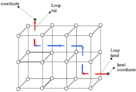
B. Closing Partial Loops

When a loop terminates on the boundary of the phase volume, it defines an open loop that needs to be closed before marking the zero-weighted edges. Let us assume that we want to close the partial loop that is shown in Fig.5.

The closing procedure can be summarized in the following steps:

1. Randomly choose one end of the loop to be the head and the other end to be the tail, as shown in Fig. 6.

2. Calculate the coordinates of the head and the tail, which are shown in Fig. 6.

3. Identify the five artificial residues that can po-tentially be connected to the tail residue in three di-mensions. For clarity in our example, Fig.7(a)shows only three out of the total of five possible artificial residues that may be connected to the tail. The other two potential residue paths, namely, those perpen-dicular to the plane of the page, i.e., located in directions moving both into and out of the page, re-spectively, have been left out here as they would obscure the diagram.

4. Calculate the coordinates of the five residues that were identified in step 3.

5. Calculate the distance between each artificial residue and the loop head.

6. Choose the artificial residue that has the mini-mum Euclidian distance to the head of the loop to be connected to the loop. If two residues have the same distance, then one of these residues is arbitrarily connected to the loop. In our example, one of the artificial residues is connected to the loop as shown in Fig. 7(b).

7. Check if this artificial residue closes the loop. If yes, then the loop is closed and this procedure is ended. Otherwise continue with step 8.

8. Mark this artificial residue as a new loop tail and go back to step 2 and repeat the process until the loop is closed.

Figure 7(c) shows the resulting fully closed loop after carrying out the procedure described above.

C. Identifying Zero-Weighted Edges

Once singularity loops have been identified, the algo-rithm proceeds to identify the zero-weighted edges, i.e., those edges that penetrate the singularity loops. The idea behind this procedure depends on grad-ually shrinking a loop toward its center until it vanishes. As the loop shrinks, it passes through suc-cessive edges. Each time this happens, the edge is permanently marked as a zero-weighted edge. The procedure of shrinking the loop is based on finding and processing the individual U-shaped and L-shaped segments which make up the body of the loop itself. U-shaped segments consist of three successive residues that form a U shape, as shown in Fig.8(a). Meanwhile, L-shaped segments consist of only two successive residues forming an L shape, as illus-trated in Fig. 8(b).

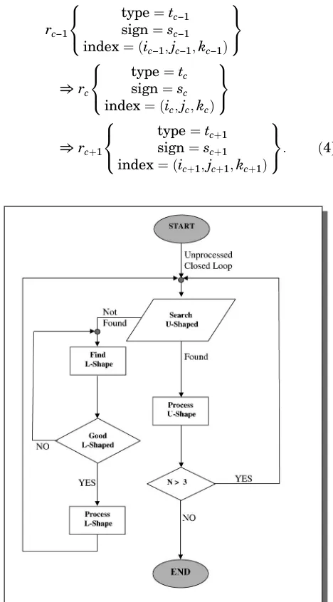
The procedure for processing a closed loop is shown in the form of a flow chart in Fig.9. First, the loop is examined to find out if it contains any U-shaped seg-ments. If a U-shaped segment is discovered, the three residues that form the U-shaped segment are replaced by the appropriate single residue value and the edge inside that U shape is marked as being a zero-weighted edge. After replacing a U shape by a single artificial residue value, the residues that re-main inside the loop are counted. If the number of residues is greater than three, the U-shape search procedure is repeated until no other U shape is discovered within the loop. Then, the algorithm searches for the first L-shaped segment that is pre-sent in the loop. If an L shape is discovered, the algo-rithm checks whether the replacement of this L shape would increase or decrease the area within that loop. If the area would be increased, then the algorithm leaves that L shape and searches for the

first“good L shape,”i.e., one that minimizes the over-all area of the loop. When a good L-shape is discov-ered, the algorithm replaces it with two new artificial residues and the edge located in between the L-shape arm is marked as a zero-weighted edge. After replacing an L shape, the algorithm again searches for a U shape. This process will be repeated until the number of residues within the loop reaches a value of less than three [20,22].

1. Detecting U-Shaped Segments

Suppose that r_c−1, r_c, and r_cþ1 are three successive residues that exist in a closed loop, where their types

Fig. 7. (Color online) Demonstration of closing partial loops. Fig. 6. (Color online) Example of a partial singularity loop that

and signs and indices are given by

rc−1 8 < :

type¼t_c−1 sign¼s_c−1 index¼ ði_c−1;j_c−1;k_c−1Þ

9 = ;

⇒rc

8 < :

type¼t_c sign¼s_c index¼ ðic;jc;k_cÞ

9 = ;

⇒rcþ1

8 < :

type¼t_cþ1 sign¼s_cþ1 index¼ ði_cþ1;j_cþ1;k_cþ1Þ

9 =

;: ð4Þ

The type variable may take one of the following values:r_x,r_y, orr_z. Thesignvariable may be assigned a þ1 or −1 value. These three residues form a U-shaped segment, if and only if, they obey the follow-ing rules:

8 < :

rc−1:type¼rcþ1:type≠rc:type rc−1:sign¼−rcþ1:sign

∥rc−1:index−rcþ1:index∥¼1 9 =

;: ð5Þ

If all the above conditions are true for the three re-sidues, then these three residues form a U-shaped segment and should be replaced in a manner to be explained shortly.

2. Detecting L-Shaped Segments

Suppose thatr_candr_cþ1are two successive residues in a closed loop, where their types and signs and indices are given by

rc

8 < :

type¼t_c

sign¼s_c

index¼ ðic;jc;k_cÞ

9 = ;

⇒rcþ1

8 < :

type¼t_cþ1

sign¼s_cþ1

index¼ ði_cþ1;j_cþ1;k_cþ1Þ

9 =

;: ð6Þ

These two residues form an L-shaped segment if

rc:type≠r_cþ1:type

ð7Þ

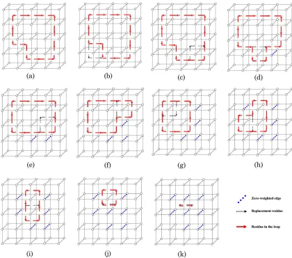
3. 3DBPASL Algorithm in Action

An example is now given to clarify the operation of the 3DBPASL algorithm. Suppose that the closed singularity loop shown in Fig.10(a)is to be processed by the procedure that has been described previously. First, the algorithm searches for any U-shaped segments located in that loop. This particular ex-ample of a closed singularity loop does not contain any U-shaped segments at this stage, so the algo-rithm then searches for any L-shaped segments. Suppose that the algorithm finds the L-shaped seg-ment that is shown in Fig.10(b). The algorithm will check if the replacement of this L-shaped segment will increase or decrease the area within the loop. The new possible choice of path for the L-shaped seg-ment that is to be replaced is shown in Fig.10(b)as marked by dotted arrows. Clearly, this possible repla-cement of the L-shaped segment will increase the overall loop area, so the procedure will ignore this choice of L-shaped segment and will continue to search for another L-shaped segment that will de-crease the entire area of the loop (this latter kind of L-shaped segment that shrinks the overall loop area will be referred to as a “good L-shaped”

seg-Fig. 8. (Color online) (a) U-shaped segment and (b) L-shaped segment.

ment). As the procedure continues, it will search

for new L-shaped segments. Figure 10(c) shows a

new L-shaped segment that has subsequently been found, and the potential replacement L-shaped segment is shown in Fig.10(c)as marked by dotted arrows. This L-shaped segment is considered to be a good L-shaped segment, because its replacement will decrease the entire area of the loop. In this case, the algorithm will replace this L-shaped segment and will mark the edge that the loop passes through dur-ing its shrinkdur-ing process as a zero-weighted edge, marked as a dotted line edge in Fig.10(d).

After replacing an L-shaped segment, the algo-rithm will again examine the loop to detect the po-tential presence of any U-shaped segments. In our case, the algorithm will find the U-shaped segment which is shown in Fig. 10(d). The potential replace-ment of this triple-residue U-shaped segreplace-ment is with a single residue only, which will definitely minimize the area of the loop, so the algorithm will directly re-place this U-shaped segment by its rere-placement and will mark the appropriate edge as a zero-weighted edge, as is shown in Fig.10(e).

After replacing the U-shaped segment and mark-ing the appropriate edge as a zero-weighted edge, the

algorithm will check the number of residues in the loop. If the number of residues in the loop is less than three, then the processing is completed for this loop and the algorithm has to identify a new closed loop to process it. In our example, the number of residues in the loop shown in Fig. 10(e) is 10, i.e., a value greater than three, so the algorithm will search for a U-shaped segment once again. Clearly, as shown in Fig.10(e), the loop does not contain any U-shaped segments, so the technique will proceed by finding the next good L-shaped segment, which it does. This is illustrated by the segment marked by dotted ar-rows in Fig.10(e). The L-shaped segment will be re-placed and the appropriate edge will be marked as a zero-weighted edge, as shown in Fig.10(f). Again, the algorithm now will search for a U-shaped segment and will replace it with its equivalent single residue value, as shown in Figs.10(f)and 10(g).

This process will be repeated many times until the whole loop is processed. Figures10(g)–10(k)show the stages of shrinking the sampled loop until the whole loop is processed and all zero-weighted edges asso-ciated within the original loop have been identified, as shown in Fig.10(k).

4. Replacement of a U-Shaped Segment

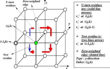
As illustrated in the example shown in Fig. 10(d), only one artificial residue is needed to replace a shaped segment. However, when replacing a U-shaped segment a number of questions arise: such as what is the type, sign, and index of the new resi-due? What is the direction of the edge that needs to be marked as a zero-weighted edge? And finally, what is the index of the zero-weighted edge? To answer these questions, several examples are now presented.

Example 1:

Figure 11 shows a U-shaped segment located in

thezxplane that needs to be replaced. This U-shaped segment consists of the following residues:

rc−1 8 < :

type¼x sign¼ þve index¼ ði;j;kÞ

9 = ;⇒rc

8 < :

type¼z sign¼−ve index¼ ði;j;kÞ

9 = ;

⇒rcþ1

8 < :

type¼x sign¼−ve index¼ ði;j;k−1Þ

9 = ;: ð8Þ

Note that these three residues obey the U-shaped rules defined in Eq. (5). As shown in Fig. 11, the new artificial residue needed to replace the U-shaped segment that is shown as a double-line arrow in the figure is given by

rn

8 < :

type¼z sign¼−ve index¼ ði−1;j;kÞ

9 =

;: ð9Þ

On the other hand, the edge needed to be marked as a zero-weighted edge, represented by a dotted line in the figure, is given by

zwe

type¼y index¼ ði;j;kÞ

: ð10Þ

This means that the edge connected between the

vox-elsði;j;kÞand (i,jþ1,k) has to be marked as a zero-weighted edge. (Note that if the type of this edge was an“xtype,”rather than the“ytype”that is given in this example, then for this case it would be the edge that connects voxelði;j;kÞwith voxel (iþ1,j,k), which has to be marked as the zero-weighted edge). From this example, we can conclude that the new residue inherits the type and sign of the middle re-siduer_c. Furthermore, the type of the zero-weighted edge that must be marked is that type that is missing from the U-shaped segment. In other words, by defi-nition the U-shaped segment will contain only two of the three possible types of residue, and the type of the zero-weighted edge will be set to the other third possible type that is not present in the U-shaped seg-ment. This is expressed in the following equations:

rn:type¼rc:type; ð11Þ

rn:sign¼rc:sign; ð12Þ

zwe:type≠ðrc:type or r_c1:typeÞ: ð13Þ

Two more questions still need to be answered: the first is how to know the index of the new residue, and the second is how to know the index of the zero-weighted edge. These two questions are investigated further in the following examples.

Example 2:

In this example we consider the U-shaped residues shown in Fig.12. These residues are given by

rc−1 8 > < > :

type¼z

sign¼−ve

index¼ ði;j;kþ1Þ 9 > = > ;⇒rc

8 > < > :

type¼x

sign¼−ve

index¼ ði;j;kÞ

9 > = > ;

⇒rcþ1

8 > < > :

type¼z

sign¼ þve

index¼ ði−1;j;kþ1Þ 9 > = >

;: ð14Þ Fig. 11. (Color online) Example 1 of replacing U-shaped

segments.

In this case, the new residue and the zero-weighted edge are

rn

8 < :

type¼x sign¼−ve index¼ ði;j;kþ1Þ

9 =

;; ð15Þ

zwe

type¼y index¼ ði;j;kþ1Þ

: ð16Þ

As seen in this example, the type and sign of the new residue still inherits the type and sign of the middle residuer_c. Also, the type of the zero-weighted edge still obeys the rule explained in the first example. By careful consideration of the index of the new re-sidue in the first and second examples, it can be no-ticed that the distance between the new residue and the middle residue,r_c, is always equal to 1. Or as a formula we can write

∥rc:index−rn:index∥¼1: ð17Þ

We refer to the index of the middle residue r_c as

ði;j;kÞin both examples. In the first example, the in-dex of the new residue is (i−1,j,k). We can note that the change in the index occurred here in thex coor-dinate, and the type of the first (or last) residue was of the x type (note that the first and the last resi-due have the same type in the U-shaped segment). Furthermore, in the current example, the new resi-due index is (i,j,kþ1), and the type of the first (or last) residue in the U-shaped segment is of theztype. From these two examples, we can conclude that

rn:index¼

8 < :

iλx jλy kλz

9 =

;; ð18Þ

where

λx¼

1; ifr_cþ1:type¼x

0; otherwise ; ð19Þ

λy¼

1; ifr_cþ1:type¼y

0; otherwise ; ð20Þ

λz¼

1; ifr_cþ1:type¼z

0; otherwise : ð21Þ

We still have to determine in which cases we have to add the lambda values and in which cases we have to subtract them. These issues are further investigated by considering more examples.

Example 3:

In this example, we consider a U-shaped segment

located in the xy plane, as shown in Fig. 13(a).

Figure13(b)shows a top view of the segment shown in Fig. 13(a).

The U-shaped residues are

rc−1 8 < :

type¼x sign¼−ve index¼ ðiþ1;j−1;kÞ

9 = ;

⇒rc

8 < :

type¼y sign¼ þve index¼ ði;j;kÞ

9 = ;

⇒rcþ1

8 < :

type¼x sign¼ þve index¼ ðiþ1;j;kÞ

9 =

;: ð22Þ

The new residue, as shown in the figure, is

rn

8 < :

type¼y sign¼ þve index¼ ðiþ1;j;kÞ

9 =

;: ð23Þ

The zero-weighted edge in this example is

zwe

type¼z index¼ ðiþ1;j;kÞ

: ð24Þ

In this example, we attempt to illustrate how to cor-rectly decide whether to add 1 to the index or whether we have to subtract 1 from the index. By looking at all the examples, we can conclude that the addition or subtraction is a function of the sign of the third residue in the U-shaped segment. When the sign of r_cþ1 is positive, then we have to add

lambda, and whenever that sign is negative we have to subtract lambda, as is the case for all three of the above examples. So, as a general rule, the index of the new residue can be calculated by

rn:index¼

8 < :

iþλx×ðrcþ1:signÞ

iþλy×ðrcþ1:signÞ

iþλz×ðrcþ1:signÞ 9 =

;; ð25Þ

whereλ_x,λ_y, and λ_z are defined by Eqs. (19)–(21). In the previous examples, we concluded how to determine the type, sign, and index for the new re-placement residue. Moreover, we also determined how to calculate the type of the zero-weighted edge that is to be marked. This leaves us with only one question still pending: What is the index of the zero-weighted edge? An additional example is con-sidered to illustrate this issue.

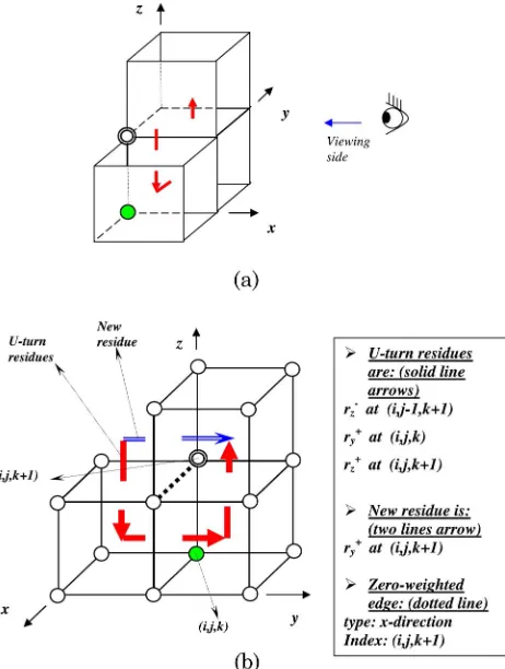
Example 4:

The U-shaped residues in this example are shown in Fig. 14(a). Figure 14(b) shows a side-on view of Fig. 14(a) for clarity. The residues forming this U-shaped segment are

rc−1 8 < :

type¼z sign¼−ve index¼ ði;j−1;kþ1Þ

9 = ;

⇒rc

8 < :

type¼y sign¼ þve index¼ ði;j;kÞ

9 = ;

⇒rcþ1

8 < :

type¼z sign¼ þve index¼ ði;j;kþ1Þ

9 =

;: ð26Þ

Using the rules defined by Eqs. (11), (12), and (25), we can conclude that

rn

8 < :

type¼y sign¼ þve index¼ ði;j;kþ1Þ

9 =

;: ð27Þ

This result matches the new residue shown in Fig.14(b). From Fig.14(b), the zero-weighted edge is

zwe

type¼x index¼ ði;j;kþ1Þ

: ð28Þ

From all the examples given above, we can see that the index of the zero-weighted edge is always equal to the index of one of the side residues in the U-shaped segment, r_c−1 or r_cþ1. Furthermore, we can note that if the sign of the middle residue r_cis positive, then the index of the zero-weighted edge is equal to the index of the last residue in the U-shaped segment, r_cþ1. In contrast, if the sign of the middle residue r_c is negative, then the index of the zero-weighted edge is the same as the index of the first residue in the U-shaped segment, r_c−1. As a result, we can summarize the rules for replacing

U-shaped segments as follows: Given the following U-shaped segment,

rc−1⇒rc⇒rcþ1; ð29Þ

the new residuer_nneeded to replace that segment is

rn:type¼rc:type; ð30Þ

rn:sign¼rc:sign; ð31Þ

rn:index¼

8 < :

iþλx×ðrcþ1:signÞ

jþλy×ðrcþ1:signÞ

kþλz×ðrcþ1:signÞ 9 =

;; ð32Þ

where

λx¼

1; ifr_cþ1:type¼x

0; otherwise ; ð33Þ

λy¼

1; ifr_cþ1:type¼y

0; otherwise ; ð34Þ

λz¼

1; ifr_cþ1:type¼z

0; otherwise : ð35Þ

The edge that needed to be marked as a

weighted edge is determined by

zwe:type≠ðrc:type or r_cþ1:typeÞ; ð36Þ

zwe:index¼

rc−1:index ifrc:sign¼−ve

rcþ1:index ifrc:sign¼ þve: ð37Þ

5. Replacement of L-Shaped Segments

Replacement of the L-shaped segments can be carried out by depending on the rules for U-shaped segments that were presented in Subsection 4.C.4. Suppose that we want to replace the L-shaped residue pair, denoted as r_c and r_cþ1 in Fig. 15, by two new artificial residues r_n1 and r_n2 as shown in the figure.

From Subsection4.C.4, we concluded that the new artificial residue is determined by the center and the last residues in the U-shaped segment, i.e., r_c and rcþ1. This conclusion can be applied in the case of

L-shaped residues. As shown in Figs.16(a)and16(b), the artificial residue r_n2 in the case of an L-shaped residue is equivalent to the residue r_n in the U-shaped segment, so residuer_n2can be determined as ifr_c andr_cþ1 form part of a U-shaped segment.

After determiningr_n2, the residuer_n1can be deter-mined by consideringr_c,r_cþ1, andr_n2as a U-shaped segment, as shown in Fig.16(c). Note thatr_n2has the opposite sign to r_n2. As a result, we can summarize the rules for replacing an L-shaped segment as follows: Given the following L-shaped segment,

rc⇒rcþ1; ð38Þ

the new artificial residuesr_n1andr_n2are determined by three steps:

Step 1: following the U-shaped rules, find r_n2 fromr_c⇒r_cþ1;

Step 2: from r_cþ1⇒r_n2 find r_n1, where

rn2:type¼rn2:type; ð39Þ

rn2:sign¼−rn2:sign; ð40Þ

rn2:index¼rn2:index; ð41Þ

Step 3: find the correspondingzwefromr_c⇒r_cþ1 following the U-shaped rules defined in Eqs. (36) and (37).

D. Calculating the Edge Qualities

After identifying all the zero-weighted edges in the wrapped phase volume, the algorithm sets the qual-ity values for these edges to zero. Then the algorithm proceeds to calculate the quality values for each individual remaining edge in the phase volume. The calculation of these qualities is carried out using the second difference method that is explained in [19]. Afterward, all the edges are sorted in an order according to descending quality values. Finally, the unwrapping process is carried out using the 3D best-path phase-unwrapping algorithm, as was described in Section2.

5. Results and Comparisons

To evaluate the performance of the proposed algo-rithm, two different kinds of wrapped-phase volume were processed, namely, computer-generated and real wrapped-phase volumes, respectively. Both of these types of phase volumes were unwrapped using the proposed technique. The 3DBPASL algorithm was then compared with both the noise-immune [15] and the best-path algorithms [19], respectively. A comparison with Cusack’s algorithm [13] has also been provided to enrich our assessment. The results show that the proposed 3DBPASL algorithm outper-forms all the other algorithms in terms of robustness and reliability.

A. Computer Simulation Results

The proposed algorithm has been tested using a computer-simulated wrapped phase volume, which was generated as follows. The computer-generated dynamic object used here is a complicated surface whose shape is changing with time, i.e., with the

frame number. Each frame consists of 256×256

pixels. The shape of this surface at timetis given by

Fig. 15. (Color online) L-shaped segment and its replacement.

zði;j;tÞ ¼10×

σ1ðtÞ·sin½xði;jÞ

xði;jÞ þσ2ðtÞ·

sin½yði;jÞ yði;jÞ

;

ð42Þ

where xði;jÞ and yði;jÞ are defined in the range

½0;255and they refer to the pixel indices. The term zði;j;tÞ is the height of the pixel ði;jÞ at time t

(actually, here t represents the frame number).

The termsσ1ðtÞandσ2ðtÞare time varying functions that are given by

σ1ðtÞ ¼1:50−ð0:01×ðtþ1ÞÞ; ð43Þ

σ2ðtÞ ¼0:49þ ð0:01×ðtþ1ÞÞ; ð44Þ

wheret is defined in the range½0;99.

This computer-generated moving object is repre-sented using 100 two-dimensional video frames, each consisting of256×256pixels, thereby representing a total 3D data volume of256×256×100voxels. To in-crease difficulty and add realism to this simulated test, a 16-frame region of noise is embedded within the overall data volume, beginning at frame 47 and ending at frame 62. This noisy volume therefore con-sists of256×256×16voxels, which have a Gaussian noise profile with zero mean and a standard devia-tion of 1.55. The presence of this region of noise may provoke unwrapping errors and should enable us to test for any potential error propagation into the third

“clean” region of wrapped phase data. Then, the whole phase volume is wrapped between the values

of −π and þπ using the mathematical arctangent

function. Hence, the wrapped phase volume appears to be divided into three discrete sets. The first and third sets are clean simulated wrapped phase vo-lumes (the first set running from frame 0 to frame 46 and the third set running from frame 63 to frame 99). The second set (running from frame 47 to frame 62) is a noisy region whose quality is degraded by the addition of noise as described above.

The whole resulting wrapped phase volume was

then unwrapped using Cusack’s algorithm, the

PRELUDE unwrapper, Huntley’s algorithm, the

3D best-path algorithm, and the proposed 3DBPASL algorithm. The results are shown in Fig.17using a range image representation (with the color white representing the maximum value in the image and black representing the minimum value).

Row (a) in Fig.17shows a single sample wrapped phase map from each of the three different wrapped phase regions. The first map (the left-most) corre-sponds to frame number 46 (which lies in the first region), the second to frame number 55 (in the second noisy region), and the third to frame 84 (in the third region).

Row (b) in Fig. 17 shows the unwrapped phase

maps that were produced using Cusack’s algorithm. It can be observed that although this algorithm suc-ceeds at unwrapping frames 46 and 84, it fails to un-wrap frame 55 (lying within the noisy region).

Despite this failure, the algorithm has been able to isolate the noisy region and prevent error propaga-tion throughout the entire phase volume. This result is due to the fact that it relies upon a quality measure to guide the unwrapping procedure. This quality measure assigns lower qualities to those voxels lo-cated in the noisy region and thus this region was unwrapped last.

Row (c) shows the unwrapped phase maps gener-ated using the PRELUDE algorithm. The visual in-spection of the results illustrates that the algorithm succeeded in unwrapping the phase volume, but the resultant unwrapped phase maps that correspond to

clean wrapped frames are noisy. This reveals that the PRELUDE unwrapper could not prevent errors from propagating from noisy frames to clean frames.

The results for Huntley’s algorithm are shown in Fig.17, row (d). As shown in these images, Huntley’s algorithm succeeds at unwrapping frames 46, 55, and 84, and it also manages to produce a fair result at unwrapping the noisy frame. Huntley’s algorithm performs better than Cusack’s algorithm in attempt-ing to unwrap frame 55, thereby exhibitattempt-ing higher robustness against noise.

Row (e) shows the results for the 3D best-path

phase-unwrapping algorithm. This algorithm

succeeds at identifying the noisy region and mini-mizes error propagation. The algorithm unwraps frames 46 and 85 successfully, without being affected by the presence of the noisy region. The algorithm also produces reasonable results when unwrapping the noisy region, as is shown in the middle frame of this row. However, it is worth noting that Huntley’s algorithm manages to produce a better unwrapped phase map for frame 55 (lying within the noisy re-gion) than is the case for the best-path algorithm.

The results for the proposed 3DBPASL approach are shown in row (f). The 3DBPASL algorithm pro-vides better results than any of the other algorithms. It not only successfully isolates the noisy region and processes it last, but also gives good results when un-wrapping those frames that lie within the noisy region.

B. Experimental Results

The proposed phase-unwrapping algorithm was also tested experimentally, i.e., involving real wrapped phase data. This test was performed by measuring a dynamically moving RANDO phantom (a synthetic human head and torso used in radiotherapy calibra-tion) undergoing manually induced pseudorespira-tory motion in a laborapseudorespira-tory setting. Fringe patterns were projected onto the phantom’s face. The deformed fringe patterns were captured using a CCD camera and they form a video sequence, which was subse-quently analyzed using the Fourier fringe analysis technique thereby producing a real experimental wrapped phase volume [10]. The wrapped phase

volume so obtained had dimensions of 512×512×

25 voxels, and this was then unwrapped using the

proposed 3DBPASL algorithm and the other 3D comparative algorithms.

Row (a) in Fig.18, reading from left to right, shows the respective wrapped phase maps taken from frames 0, 15, and 24 of the wrapped phase volume. The unwrapped phase maps that were produced using the Cusack algorithm, the PRELUDE rithm, the Huntley algorithm, the best-path algo-rithm, and the 3DBPASL algorithm are shown in rows (b), (c), (d), (e), and (f), respectively. As the figure shows, Cusack’s algorithm and the best-path algo-rithm both give very poor results. Huntley’s algo-rithm is still robust at dealing with noise, but

ambiguities in the singularity loops have produced a separated region near the dummy’s nose.

The results of the proposed 3DBPASL approach are shown in Fig.18(f). This new technique produces better results than the other three comparative tech-niques presented here. The 3DBPASL algorithm is capable of finding an optimal path, while taking ad-vantage of the fact that it also processes and avoids singularity loops. Although ambiguities still exist in the singularity loops that are identified by this algo-rithm, the effect of these ambiguities is minimized

because of the fact that here we are also using a qual-ity map to guide the unwrapping path.

In this work the 3DBPASL algorithm has been pro-grammed in the C computer language. The C code used to obtain the results presented in this paper is freely publicly available, subject to nonprofit making conditions, and is published on our website [23].

The five phase-unwrapping algorithms mentioned above were executed on a host computer platform with a Pentium 4 processor and 4GRAM. The execu-tion times for these five algorithms were measured by processing the entire 512×512×25voxel phase volume for the RANDO phantom on this computing platform. The execution times for the Huntley, Cusack, 3D best-path, and 3DBPASL algorithms were of the order of30s; whereas the execution time for the Prelude algorithm was of the order of 3 days.

6. Conclusion

A novel three-dimensional phase-unwrapping algo-rithm has been proposed that we have referred to as the three-dimensional best-path avoiding singu-larity loops (3DBPASL) algorithm. This technique has been shown to be robust and is a hybrid algo-rithm combining the 3D noise-immune phase-un-wrapping algorithm proposed by Huntley with the 3D best-path algorithm. The 3DBPASL algorithm finds an optimal unwrapping path, while also taking into account the effect of singularity loops. This is performed by using zero-weighted edges to adjust the optimal path and avoid these singularity loops. The 3DBPASL algorithm has an important ad-vantage over the 3D noise-immune algorithm. The 3D noise-immune algorithm does not consider the quality of each individual voxel and, although it iden-tifies and processes singularity loops, ambiguities may be present in these loops which may cause error propagation. On the other hand, the 3DBPASL not only identifies these singularity loops, but it also cal-culates the quality of each voxel to ensure that the most reliable voxels are unwrapped first and thus the effects of singularity loop ambiguities are mini-mized or removed entirely.

The algorithm has been tested by using both computer-simulated and real wrapped phase vol-umes, and it has demonstrated high robustness le-vels and high lele-vels of immunity against noise. The 3DBPASL algorithm has been compared with other state-of-the art, robust, 3D phase-unwrapping rithms. Results have shown that the proposed

algo-rithm outperforms these other state-of-the-art

algorithms, producing improved results.

References

1. D. C. Ghiglia and M. D. Pritt, Two-Dimensional Phase Unwrapping: Theory, Algorithms and Software(Wiley, 1998). 2. M. D. Pritt and J. S. Shipman,_“Least-square two-dimensional phase unwrapping using FFTs,_”IEEE Trans. Geosci. Remote Sens.₃₂, 706_–708 (1994).

3. D. C. Ghiglia and L. A. Romero, _“Minimum _Lp-norm two-dimensional phase unwrapping,_” J. Opt. Soc. Am. ₁₃, 1999_–2013 (1996).

4. R. Cusack, J. M. Huntley, and H. T. Goldrein, _“Improved noise-immune phase-unwrapping algorithm,_”Appl. Opt.₃₄, 781_–789 (1995).

5. S. A. Karout, M. A. Gdeisat, D. R. Burton, and M. J. Lalor, “Two-dimensional phase unwrapping using a hybrid genetic algorithm,_”Appl. Opt.₄₆, 730_–743 (2007).

6. M. Arevalillo Herráez, D. R. Burton, M. J. Lalor, and D. B. Clegg,_“Robust, simple, and fast algorithm for phase un-wrapping,_”Appl. Opt.₃₅, 5847_–5852 (1996).

7. W. Xu and I. Cumming, _“A region-growing algorithm for InSAR phase unwrapping,_”IEEE Trans. Geosci. Remote Sens. 37, 124_–134 (1999).

8. M. Arevalillo Herráez, D. R. Burton, M. J. Lalor, and M. A. Gdeisat, _“Fast two-dimensional phase unwrapping algorithm based on sorting by reliability following a non-continuous path,_”Appl. Opt.₄₁, 7437_–7444 (2002).

9. K. Stetson, J. Wahid, and P. Gauthier,_“Noise-immune phase unwrapping by use of calculated wrap regions,_”Appl. Opt.₃₆, 4830_–4838 (1997).

10. F. Lilley, M. J. Lalor, and D. R. Burton,_“Robust fringe analysis system for human body shape measurement,_”Opt. Eng.₃₉, 187_–195 (2000).

11. M. Costanitini, F. Malvarosa, L. Minati, and G. Milillo, “A three dimensional phase unwrapping algorithm for proces-sing of multitemproral SAR interferometric measurements,_” IEEE Trans. Geosci. Remote Sens.₄₀, 1741_–1743 (2002). 12. H. S. Abdul-Rahman, M. A. Gdeisat, D. R. Burton, M. J. Lalor,

F. Lilley, and A. Abid, _“Three-dimensional Fourier fringe analysis,_”Opt. Las. Eng.₄₆, 446_–455 (2008).

13. R. Cusack and N. Papadakis,_“New robust three-dimensional phase unwrapping algorithm: application on magnetic field mapping and undistorting echo-planar images,_”NeuroImage 16, 754_–764 (2002).

14. X. Su, W. Chen, Q. Zhang, and Y. Chao,_“Dynamic 3D-shape measurement method based on FTP,_” Opt. Las. Eng. ₃₆, 49_–64 (2001).

15. J. M. Huntley, _“Three-dimensional noise-immune phase unwrapping algorithm,_”Appl. Opt.₄₀, 3901_–3908 (2001). 16. M. Jenkinson,_“Fast, automated, N-dimensional phase

unwrap-ping algorithm,_”Magn. Reson. Med.₄₉, 193_–197 (2003). 17. H. S. Abdul-Rahman, M. A. Gdeisat, D. R. Burton, and

M. J. Lalor, _“Fast three-dimensional phase unwrapping algorithm based on sorting by reliability following a non-continuous path,_”Proc. SPIE₅₈₅₆, 32_–40 (2005).

18. H. S. Abdul-Rahman, M. A. Gdeisat, D. R. Burton, and M. J. Lalor, _“Three-dimensional phase unwrapping algo-rithms: a comparison,_”presented at the Photon06 Conference, Manchester, UK, 4_–7 Sept. 2006.

19. H. S. Abdul-Rahman, M. A. Gdeisat, D. R. Burton, M. J. Lalor, F. Lilley, and C. Moore,_“Fast and robust three-dimensional best-path phase unwrapping algorithm,_” Appl. Opt. ₄₆, 6623_–6635 (2007).

20. O. Marklund, J. Huntley, and R. Cusack,_“Robust unwrapping algorithm for three-dimensional phase volumes of arbitrary shape containing knotted phase singularity loops,_” Opt. Eng.₄₆, 085601 (2007).

21. M. Salfity, P. Ruiz, J. Huntley, M. Graves, R. Cusack, and D. Beauregard,_“Branch cut surface placement for unwrap-ping of undersampled three-dimensional phase data: applica-tion to magnetic resonance imaging arterial flow mapping,_” Appl. Opt.₄₅, 2711_–2722 (2006).

22. H. S. Abdul-Rahman, _“Three-dimensional Fourier fringe analysis and phase unwrapping,_”PhD thesis (Liverpool John Moores University, 2007).