Understanding Economic Growth in Indian States

Munich Personal RePEc Archive

Understanding Economic Growth in

Indian States

NR, Bhanumurthy

15 May 2009

IEG Discussion Paper Series No.137/2009

Understanding Economic Growth in Indian States

By

N R Bhanumurthy & Prakash Singh

*

Abstract

The present study tries to understand the trends and determinants of economic growth in Indian states. For this, it considers two important determinants such as infrastructure and financial development. With the help of panel time series models, the study concludes that although both the variables are highly correlated with economic growth, it is the social sector development that is having higher impact on the economic growth. In terms of the role of financial sector, the results show that although it is necessary to have development in terms of increase in number of bank branches, it is the extent of bank business that is more important in the growth process.

Key Words: Economic Growth, Infrastructure, Financial Development, Panel Time Series, India. JEL Classification: H54, N20, F43 and O16

* N R Bhanumurthy & Prakash Singh are Associate Professor and Senior Research Analyst, respectively,

Understanding Economic Growth in Indian States

Introduction

India’s recent success in growth and its sources have been widely discussed and debated

both in academic and policy circles extensively. But the conclusions regarding the timing,

pace and the determinants of the structural shift in overall economic growth is rather

inconclusive (see Balakrishnan & Parameswaran (2007a, b), Rodrik &

Subramanian(2005), Bosworth et al. (2007) and these are only a selected studies). Most

of these studies have attempted to explain this growth story with the help of standard

growth theories and its variants such as endogenous growth schools. There are other set

of studies that have shown that indeed these high growth phase has also resulted in

widening regional disparities at the state level (Ahluwalia (2000), Rao, et al. (1999)). To

some extent this conclusion has been widely accepted and has been discussed at the

policy level to reduce the spatial disparities emanating in the growth process. The

Eleventh Five Year Plan’s focus of achieving “inclusive growth” is in itself major

evidence that the regional divergences are quite severe and are in need of immediate

policy responses. Towards this direction, the Indian Planning Commission, in the current

Five year plan, is re-emphasizing micro approach by focusing more on the District level

planning process through establishing District Planning Committees. But, unlike at the all

India level, there are not many rigorous studies at the state level that examines the

underlying determinants of economic growth in the recent period. At the District level,

the unavailability of output data restricts any such studies.

Towards this direction, the present study makes an attempt to examine the timing, pace

and determinants of economic growth at the state level. In particular, the study would

examine the role of infrastructure faculties and financial sector development and its reach

at the state level growth process. In the theoretical literature, these two factors have been

identified as the major determinants for enhancing growth atleast in the developing

countries. Even at the all India level, the Eleventh Plan does focus on these two factors to

stimulate growth. At the empirical level, there are many cross-country studies that have

Some studies have even showed that the growth achieved through improvement in these

factors would have more potential to reduce poverty and inequality.

The rest of the paper is organized as follows. In the next section, the analytical

framework that is adopted in the study would be discussed. In section-3, the details about

the database, preliminary results about the trends and behavior of state GDP,

infrastructure and financial indicators would be discussed. A brief description about the

methodology adopted in the study would be presented in Section-4. Structural shifts in

the state GDP would be discussed in section-5. In section-6, econometric results

regarding the impact of infrastructure and finance at the state level would be dealt. The

last section would draw conclusions.

Analytical Framework for the study

Taking from Barro (1990) and Hulten, et al. (2005), to examine the effect of social and

physical infrastructure and financial development at state level in India, the analytical

framework for this study uses a production function approach wherein both infrastructure

and financial development variables enter the function as in the form of capital. For this

purpose, the study adopts some variation of the Cobb-Douglas production function as

under the neo-classical framework that this production function would indeed serve as a

basic form (Jorgensen (1963)). This can be expanded by incorporating decisions

regarding investments in fixed assets such as infrastructural facilities that are expected to

improve efficiency of any production activity.

Standard production function with labour and capital as inputs are taken and extended the

same by including infrastructure and financial sector development for determining

production. Endogenous growth theory extends the definition of the word capital to

include other forms of capital such as human capital, social capital, infrastructure, and

financial capital in addition to the microeconomic definition of capital that includes

machinery i.e. physical capital and capital in form of investments. To make things

simpler, as per the requirement of the study we have not included all the measures of

financial capital. Broadly, infrastructure can be divided into physical and social

infrastructure. Physical infrastructure includes transport facility (road, rail, sea and air),

telecommunication etc, whereas education, health and sanitation etc are grouped in social

infrastructure.

In this framework infrastructure affects output in two ways; one is the direct channel

where infrastructure increases the output by reducing the cost of intermediate goods and

helps in achieving higher investments (Bougheas, et al. (2000)). For example, a proposed

business investment avenue at a proposed location will loose its viability because of the

infrastructure unavailability (transport, telecommunication etc.) but availability of

infrastructure will make the investment viable. Thus higher per capita availability of

infrastructure capital reduces the fixed cost of production. The other channel is through

externality effect. This channels works through higher human capital returns due to

education, good quality health and higher efficiency of the human capital due to lower

marginal depreciation of capital. Additionally, physical infrastructure affects the

cost/output by its effect on social infrastructure. Better physical infrastructure helps in

swelling the human capital through increasing its efficiency in turn affects output by

increasing the R&D, innovation and lower fixed cost of production.

Similar to infrastructure, the role of finance is also very crucial in any production process.

The literature on the relationship between finance and growth is vast. Although the

impact of finance on growth is not clear, it is very well established that better financial

institutions and instruments would reduce the transaction and information cost and makes

the production activity competitive and viable in the long run. Financial institution

provides incentive to restructure the market allocations in such a way that it would reduce

the fixed cost of production. Gathering information and evaluation of the firm and its

management before making any investment decision entails a huge transaction cost, thus

makes availability of funds costlier for the firms. Financial intermediaries helps in

reducing transaction cost in acquiring and processing the necessary information and helps

the better allocation of scarce resources. Further, it also helps in mobilization of savings

Weiss (1983) and Diamond (1984)). Financial sector also plays a major role in the

corporate governance. A developed financial market reduces the cost of corporate

governance compared to less developed financial sector, (Bencivenga & Smith (1993)).

This is very important from sustainability and viability point as the effectiveness of

corporate governance mechanisms directly impacts firm performance with potentially

large ramifications on national growth rates and this would largely depend on the extent

of development of financial sector.

Greenwood & Jovanovic (1990) explains the role of financial intermediaries in

accelerating growth by better allocation of resources through improved information on

firms, managers, and economic conditions, though this information is not free but the cost

is very much lower as compared to the cost incurred by individual for the same amount of

information. Besides this access to lower cost information to the investors helps them in

making better decision and thus helps the directors to oversee the managements

effectively. King & Levine (1993b) introduce financial intermediaries in growth process,

where financial intermediaries boost the rate of technological innovation through reward

to the entrepreneurs.

Considering the arguments of infrastructure-growth and finance-growth literature the

theoretical model that can be used for empirical verification of the role of infrastructure

(both physical and social) and finance in growth dynamics at state level for India is

specified below.

Y = F (IP, IS, F and L)

Y is output (State Domestic Product)

IP is expenditure on physical infrastructure

IS is expenditure on social infrastructure

F is variables reflecting financial sector development

L is labour

In general, physical infrastructure can include revenue and capital expenditure on

transport, energy and irrigation and flood control whereas, social capital includes revenue

sanitation. Increase in the social capital is supposed to have positive effect on output

through its positive long run effect on development of human capital. Similarly,

improvements in physical infrastructure capital will have positive effect on state level

output by reducing the fixed cost as well as its effect on human capital. In order to study

the effect of financial development at state level we have used number of bank branches

and credit to deposit ratio as the indicator of financial development in the absence of

typical variables of financial development at state level. Here, increases in the number of

bank branches is supposed to have positive effect on state output as increase in the

number of bank branches signifies financial inclusion and thus will have positive effect

on savings mobilization and investment. Similarly credit to deposit ratio is supposed to

have positive effect on output as increase in credit to deposit ratio indicates increase in

profitable investments. Due to unavailability of the data at the state level, we excluded

labour from the empirical model although it is integral part of growth model. All the

variables are in real terms except number of bank branches and credit to deposit ratio.

Review of Literature

In this section, as this paper addresses the issue of economic growth in Indian states and

its linkage to the development of financial sector and infrastructure, review of some of

the existing studies on finance-growth and infrastructure-growth linkages would be

undertaken.

On Finance and Growth:

It was Bagehot (1873) and Schumpeter (1912), who first explained the link between

finance and growth. Latter, number of studies has been done in this area and the role of

financial system in economic growth process has been extensively discussed. Some of

them have even studied the role of banking system separately and some have discussed

the importance of stock market in economic development. There is no dearth of studies

on both at individual country level and at the cross-country level. Diamond (1984)

highlights importance and positive role of bank based financial system in the capital

allocation process and better corporate governance by acquiring information about firms

monitoring by a financial intermediary. Rajan & Zingales (1998) modeled and explains

the role of powerful banks in debt repayment enforcements especially when the country

is having weak enforcement laws through its mutually beneficial effect on relationship

between borrowers and arm’s lengthbut they find this is only valid till there is no shock

like East-Asian financial crisis. Some studies explain the importance of banking system

in improving the efficiency of investments by managing inter-temporal and liquidity risk

involved. This increased efficiency significantly reduces the information cost and

increases the spectrum of the information (Allen & Gale (1999); Bencivenga & Smith

(1991)). Issue of economies of scale in mobilising the savings by banking sector has been

dealt by Sirri & Tufano (1995) and shows that using economies of scale banks pool large

surplus savings and help corporates in reaching optimum and efficient production point.

Market based financial system helps in improving the performance of managements as

better performance gives reward to them in the form managerial compensations and it

also exerts better governance (Jensen & Murphy (1990)). In this regard, Bhide (1993)

argues other way round, and exhibits that greater market development may hinder

corporate control and economic growth by increasing the number of times a particular

share is being sold and thus reducing the incentives to exert rigorous corporate control.

Further, Stiglitz (1985) argues that well-developed markets quickly and publicly reveal

information, which reduces the incentives for individual investors to acquire information.

Most of the popular studies by using different estimation procedures and different

variables for both bank and stock market show that development of financial sector are

positively related to economic growth (King & Levine (1993a), Demirguc-Kunt &

Levine (1996) Demetriades & Hussein (1996) Levine & Zervos (1998) Levine, Loayza &

Beck (2000) and Beck, Levine & Loayza (2000)). There are some studies which show

negative relationship between financial development and economic growth. One such

study is by Liu & Hsu (2006) which shows that financial sector development is

negatively related to growth in Japan and Korea by low efficiency of banking

system/financial intermediaries in allocating investment to profitable projects. Again in a

growth in developed countries and also in less developed countries. Even much earlier

Lucas (1988) argued that there is a negative relationship between finance and growth and

concludes that financial variable is an “over-stressed” determinant of economic growth.

Study by Fitzgerald (2006) put forward that there is no simple relationship between

financial development and economic growth. Further, there is no clear cut evidence that

financial liberalisation raise overall savings or investment rates. He also argues that rapid

pace of financial reform and opening to global capital markets can create considerable

instability despite efficiency gains, leading to a net reduction of investment and growth.

But given the preponderance of evidence from empirical works and theoretical modeling,

the role of financial system cannot be dismissed in economic growth process.

Additionally, Alfaro et al. (2004; 2006); Durham (2004) provide evidence that only

countries with well-developed financial markets gain significantly from FDI in terms of

their growth rates.

On Infrastructure and Growth:

The studies on infrastructure and growth are largely concentrated on developing and less

developed countries. And most of them are largely stresses the positive role of

infrastructure development in the overall growth and development process. In particular

the United Nations’ Millennium Development Goals (MDGs), in which the infrastructure

is the major goal, stresses the role that infrastructure plays in enhancing growth, and,

hence, reducing poverty. Dutta et al. (2007) exhibits the importance of infrastructure for

macro economic growth at the state level in a study of fourteen states in India,

particularly the role of economic infrastructure in determining the productivity. Results of

the study indicate that infrastructure plays an important role in determining the level of

investment and productivity of the industrial activity. Binswanger et al. (1989) uses

district level data for India and examine the impact of physical infrastructure on

agricultural output, and illustrates that infrastructure helps in reducing the transaction

cost, and thus promote agriculture output. Whereas, Elhance & Lakshmanan (1988) finds,

investment in infrastructure; both physical and social, helps in reduction of production

development for West Bengal, Majumdar & Mukherjee (2005) confirm the existence of

long run relationship between infrastructure and development with a strong causation

from infrastructure availability on development levels. Additionally, effect of different

facets of infrastructure seems to have different impacts on different dimensions of

development.

Following, the methodology of pioneer work of Hulten & Schwab (1991), which allows

accounting for externalities effect of infrastructure on growth exclusively, Hulten, et al,

(2006) found significant spillover effect of infrastructure on total factor productivity

(TFP) in the Indian manufacturing sector, contrary to that of the findings from Hulten &

Schwab (1991) study on U.S manufacturing sector. Study by O’Fallon (2003) though

failed to provide causal link between infrastructure investment and economic growth,

instead, provides an interesting conclusion that the impact of infrastructure on growth

depends on the initial conditions of the economy. Rodriguez (2007) clearly documents

the role of difference in infrastructure investment in increasing or decreasing the growth

rate of the economies. Empirical evidence of the Rodriguez (2007) study using a data set

of country-level infrastructure stocks for 121 countries since 1960 clearly shows that

cutbacks in infrastructure investment does have a significant effect on living standards

and productivity and thus growth rate.

In a series of papers Aschauer (1989a, 1989b and 1989c) provides evidence on high

economic return associated with investments in infrastructure. In fact, these studies

correlate the slowdown in the productivity of U.S. economy to that of decline in the

investment in the infrastructure sector. Results of these studies, where economic returns

from infrastructure investments are as high as 60%, invited series of debate about use of

production function and estimation methods in investigating the effect of infrastructure

on economic growth. According to Hulten & Schwab (1991), Evans & Karras (1994) and

also Holtz & Eakin (1994) a positive and statistically significant coefficient for a

government input in an estimated “production function” may only indicate the degree to

which increased income causes an increased level of government activities. Munnell

provide almost similar evidence on high return of infrastructure investments to that of

Aschauer (1989c). Taking infrastructure as technology, which reduces cost in the

production of intermediate inputs, Bougheas, et al. (2000) highlights the importance of

infrastructure in growth process. Ghosh & De (1998) using OLS and principal component

analysis examined infrastructure and regional growth dynamics in India. The study shows

that infrastructure do play an important role in explaining difference in growth at regional

level. Ghosh & De (2000) again found in a different study for South Asian countries that

endowment of physical capital is responsible for the difference in growth level attained.

Argy, et al. (1999) see infrastructure as a catalyst, which not only enables opportunities

for economic development but also creates future opportunities provided government

makes sound and active policy for investment in infrastructure. Though result of Canning

& Pedroni (2004) demonstrate strong and positive inducing effect from infrastructure to

economic growth but there exits vast variation in this inducing effect. They attribute this

variation to the existence of infrastructure beyond growth maximizing level. In other

words, the study is raising an issue of threshold level of infrastructure facilities. But these

findings may not be applicable to most of the developing countries as infrastructure

constraints are quite obvious.

Though most of the studies on infrastructure - growth relationship have showed positive

effect of infrastructure on economic development either directly through productivity or

through its effect on output, there are some studies which have reported negative results

of infrastructure on growth (Devarajan et al. (1996), Sanchez-Robles (1998) and Pritchett

(1996)). These studies argue that excessive amounts of transportation and communication

expenditures makes capital expenditures unproductive, which imply that

developing-country governments have been misallocating public expenditures in favor of capital

expenditures at the expense of current expenditures and Pritchett (1996) brought the issue

of public investment in unproductive projects making marginal productivity of the output

capital lower than the investment.

To sum up, the review shows that there are some mixed results regarding the impact of

case of infrastructure, although most show positive impact, there are non-linearities as

excessive investments might have negative impact. But this situation may not be same in

developing countries like India where the infrastructure deficit has been clearly identified

as one of the major factor that could hamper in sustaining high growth. Further, in the

case of financial sector also, the sector has not covered even of half of the population in

most of the developing countries. Hence, in this study, we try to examine the impact of

financial sector development and infrastructure on growth in Indian states.

Data Description:

Study uses annual data for the period 1985-86 to 2005-06. For state domestic product the

data is taken from RBI sources (Handbook of statistics on Indian economy). Trend and

Progress of Banking in India published by RBI is used for financial sector development

indicators such as number of bank branches and credit to deposit ratio at the state level by

scheduled commercial banks. For the data on infrastructure (both physical and social), we

have largely relied on the RBI report on “State Finances: A Study of Budgets”.

Following are the variables we have used in the study: SDP (real state domestic product

at 1993-94 prices in rupee crore), for economic infrastructure variable we have used

expenditure on economic infrastructure – (irrigation, energy and transport) in real

terms/deflated by WPI in rupee crore (RSOC) where as for social infrastructure we have

taken expenditure on social infrastructure – (health, education and water and sanitation)

in real terms/deflated by WPI with 1993-94 base in rupee crore) (RECO). In addition to

these variables, credit-deposit ratio of scheduled commercial banks according to point of

utilization wise (CDRUW) and number of scheduled commercial bank branches (BB) has

been used in the study to represent development in the financial sector.

Conversion of SDP series to new Base year

Use of long time series data of States’ GDP in India is an issue. The change in the base

period from 1980-81 to 1993-94 at the all India level has led to this problem. Although at

the all India level, the data on real economic activity with base 1993-94 is available even

for backwards years, but at the State level these data are not available. As the change in

index) and the production basket, simply price splicing is not sufficient. Hence, it is

necessary to shift upwards the production curve as well. As the study covers the data

from 1980-81 to 2005-06 for the estimation, we need to convert the SDP series to the

1993-94 base year from the 1980-81 base. There are two steps: first, compute the

difference in SDP for period 1993-94 between both the series with base years 1980-81

and 1993-94 for which data are available. This difference in the SDP at 1993-94 between

two series has occurred due to upward shift in the production function that includes new

economic activities and exclusion of few older activities that are extinct. Now to get the

new series on the base year 1993-94, we first assume that this shift in production has not

occurred in a single year and it is also assumed that production changes has also

happened in the year 1980-81. This difference in output, which has been accounted in the

year 1993-94, needs to be redistributed asymptotically backwards with an annual

declining rate up to year 1980-81. This can be better understood from figure-1, where E0

is the common year (here it is 1993-94) and the difference of output due to change in

production is represented by the gap E1-E0. In this case, to get the new series from

1980-81 to 1992-93, i.e., for thirteen years, we use the formula Y*1992-93=Y1992-93+(E1

-E0)*(12/13) for 1992-93, Y*1991-92=Y1991-92+(E1-E0)*(11/13) for 1991-92 and finally

Y*1980-81=Y1980-81+(E1-E0)*(1/13) , where superscript ‘*’ indicates new series. It may be

noted from the graph that the difference has been redistributed by sliding backward up to

year 1980-81 shown as dashed line, indicating a declining weight backwards for the new

economic activities in the production basket. In the next step, we compute the price

deflator with 1993-94 by simple splicing and then divide the nominal series by this

deflator to get real SDP at 1993-94 prices.

Figure-1: Shift in Production Function with change in Base year

E1

E0 A

Before we get into empirical estimations, some discussion on the trends and structural

behaviour of infrastructure, finance and growth variables is pertinent.

Trends in State indicators

Recent research on Indian states has largely focused on the issue of growth

divergence/convergence in the post-reform period. While it is largely accepted that

economic reforms in India has led to growth divergences and the public policy has started

addressing this issue, here we concentrate on the factors that determine growth at the

regional level in the endogenous growth framework. A study by Sachs et al. (2001)

shows that urbanization as the major factor in shaping the output growth at state level in

India for 15 major states. Social and demographic factors (like infant mortality rate and

adult literacy rate) were found to be explaining the standard of well-being, but found to

be weak determinant of economic growth at the state level. Rao, Shand, & Kalirajan

(1999) bring out the importance of infrastructure and human resource in determining the

level of investment at the state level and thus output growth. Nagaraj et al. (2000)

highlights the growth impact of specific types of infrastructure (like: primary education,

health conditions, irrigation, roads and rail network, power capacities, and financial

development) on the growth performance of Indian States during 1970-94. Besley &

Burgess (2000) provide evidence on the importance of land reforms as an instrument of

increasing the output growth at state level in India.

Based on the literature we find that studies on the factors that affect economic growth is

limited in the post-reform period. Although some have done in the 1990s, as the reforms

in most of states were implemented in the later half of 1990s and further there is large

heterogeneity across states, it is necessary to address this issue now with the availability

of sufficient data for empirical examination in the post-reform period. Investment on

infrastructure (both physical and social) has been focused more from the 10th Plan

onwards and in the 11th Plan the targets for infrastructure investment has been set at

more than US$500 billions under public-private partnership. Hence, it is necessary to

level in the recent period. Before getting into econometric exercise, discussion on some

trends might be useful.

Trends in financial indicators

Financial sector development in terms of credit-deposit ratio, which is likely to increase

in the post-reform period as reforms were expected to increase competition in the

banking sector and help stimulate the credit disbursement for productive investments,

shows that the process of financial reforms has not brought substantial improvement in

the credit deposit ratio in most of the states (see figure-2). Instead the ratio has either

remained same or even deteriorated in more than half of the states that are covered in this

study. It seems that there is mixed effect of financial sector reforms and has increased

inequality among the states, which could one of the reasons for widening inequality of

growth among the states in the post-reform period.

Figure-2: Comparison of Credit-Deposit Ratio

0 20 40 60 80 100 120

0 20 40 60 80 100 120

1991-92

20

0

5

-0

6

Source: Trends and Progress of Banking in India, RBI

Figure-3: Comparison of Number of Bank Branches

0 2000 4000 6000 8000 10000

0 2000 4000 6000 8000 10000

1991-92

20

0

5

-0

6

Similarly, with the introduction of new private and foreign banks, it was expected that

number of bank branches (which is used as proxy for reach/accessibility) would

alsoincrease. But there was no major increase in this variable as well during 1991-92 and

2005-06 (see figure-3). Thus, it is quite clear that banking sector in particular and

financial sector as a whole, although developed at the all India level, shows some mixed

results at the state level. This vindicates our view that the reforms at the state level are

highly heterogeneous and is expected to have differential impact on the growth at the

state level. These results are similar when the normalized variables such as credit-GDP

ratio and banks per 1000 population are used.

Figure-4: Plot of Credit to Deposit Ratio and SDP in1991-92

0 20 40 60 80 100 A n d h ra A s s a m B ih a r D e lh i G o a , G u ja ra t H a ry a n a H im a c h a l P J & K K a rn a ta k a K e ra la M a d h y a M a h a ra s h tr O ri s s a P o n d ic h e rr y P u n ja b R a ja s th a n T a m il U tt a r W e s t

CD RATIO ₀200

400 600 800 1000

SDP

CD RATIO SDP

Source: Trends and Progress of Banking in India, RBI and National Income Accounts and Statistics, CSO

Figure-5: Plot of Credit to Deposit Ratio and SDP in 2005-06

0 20 40 60 80 100 120 A n d h ra A s s a m B ih a r D e lh i G o a , G u ja ra t H a ry a n a H im a c h a l P J & K K a rn a ta k a K e ra la M a d h y a M a h a ra s h tr a O ri s s a P o n d ic h e rr y P u n ja b R a ja s th a n T a m il U tt a r W e s t

CD RATIO ₀500

1000 1500 2000

SDP

CD RATIO SDP

This trend in credit deposit ratio is found to be similar to that of the real SDP for both the

time points 1991-92 and 2005-06 (see figure- 4 and 5). A simple correlation estimates

show that the relation between credit-deposit ratio and SDP shows an increased positive

correlation from 0.41 to 0.65 between two time points (1991-92 and 2005-06). This

indicates that in states where the credit-deposit ratio is high the output in the

corresponding state is also high and vice-versa (see figure-4 and 5). Similarly the plot of

the number of bank branches and SDP shows that development of financial sector is

important for output growth (see figure 6 and 7). To understand the cause and effect

relationship, we estimate the cross-sectional regression to see the impact of credit deposit

ratio and number of bank branches on real SDP at both the points (1991-92 and 2005-06).

Regression result shows that credit deposit ratio has a positive and significant effect on

the SDP and also a substantial improvement in the effect of the credit deposit ratio on

SDP (the coefficient changed from in 1991-92 5.87 to 14.56 in 2005-06). Although the

effect of number of bank branches is positive but its coefficient is very small as compared

to that of credit deposit ratio. Increase in the value of coefficient of number of bank

branches from 0.017 in 1991-92 to 0.8 in 2005-06 shows that increased reach of banks

are important for the economic growth. Thus, cross-sectional estimation also testifies the

well established and argued effect of development in the financial sector on output.

Figure-6: Plot of Number of Bank Branches and SDP in 1991-92

0 2000 4000 6000 8000 10000 A n d h ra A s s a m B ih a r D e lh i G o a , G u ja ra t H a ry a n a H im a c h a l P J & K K a rn a ta k a K e ra la M a d h y a M a h a ra s h tr a O ri s s a P o n d ic h e rr y P u n ja b R a ja s th a n T a m il U tt a r W e s t N O OF BAN K BRAN CHES 0 200 400 600 800 1000 SDP

NO OF BABK BRANCHES SDP

Figure-7: Plot of Number of Bank Branches and SDP in 2004-05

Source: Trends and Progress of Banking in India, RBI and National Income Accounts and Statistics, CSO

Based on these figures and simple empirical estimations, one can conclude that financial

sector development is indeed highly correlated with the overall economic growth

performance of the states as it helps in providing timely and cheaper credit to the

production activities. It would also helps in channeling the scarce capital resources. It is

important to point out here that India is one of the highest saving countries in the world

and is continuously increasing over a period of time. In the following section a similar

analysis regarding the infrastructure development.

Trends in Infrastructure indicators

As in the case of financial development, similar plots have been used to understand and

investigate at primary level the changes in infrastructure (both economic and social) at

the time of reforms and now and its effect on the state output level. Figure-8 examines

changes in social infrastructure in 2004-05 compared to situation in 1991-92, the point

when reforms took place. The plot of expenditure on social infrastructure depicts

improvement in the situation of the social infrastructure in almost all the states, though

the improvement in the condition is not very huge in some states. This only indicates that

the expenditure on social sector development has increased over a period of time, which

is in line with the government’s approach in achieving the MDG goals by 2015. But one

needs to be cautious that initial conditions in India were quite low and, hence, there is a

need for further increase in social sector expenditure.

0 2,000 4,000 6,000 8,000 10,000 A n d h ra A s s a m B ih a r D e lh i G o a , G u ja ra t H a ry a n a H im a c h a l P J & K K a rn a ta k a K e ra la M a d h y a M a h a ra s h tr a O ri s s a P o n d ic h e rr y P u n ja b R a ja s th a n T a m il U tt a r W e s t N O OF BAN K BRAN CHES 0 500 1000 1500 2000 SDP

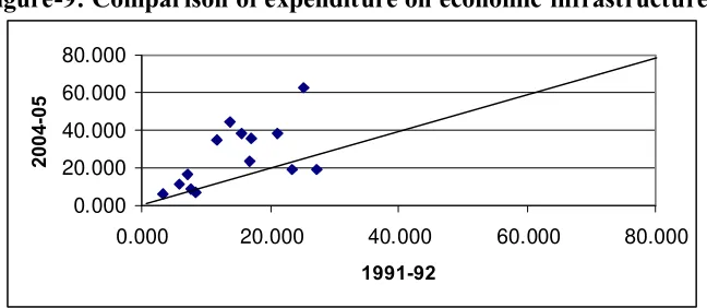
In the case of economic infrastructure, we find mixed results where the situation has

improved for some of the states but for some it has deteriorated (see figure-9). Even in

the case where the states have shown improvement they are not very substantial.

Figure-8: Comparison of expenditure on social infrastructure

0.000 20.000 40.000 60.000 80.000

0.000 20.000 40.000 60.000 80.000

1991-92

20

0

4

-0

5

Source: State Finances: A Study of Budgets and National Income Accounts and Statistics, CSO

Figure-9: Comparison of expenditure on economic infrastructure

0.000 20.000 40.000 60.000 80.000

0.000 20.000 40.000 60.000 80.000

1991-92

20

0

4

-0

5

Source: State Finances: A Study of Budgets and National Income Accounts and Statistics, CSO

It has been perceived by many that ‘infrastructure deficit’ would be a major deterrent

sustenance of current high economic growth in India. But, in our view, more important is

[image:19.612.170.512.155.297.2]

the ‘infrastructure inequality’ could be a bottleneck for balanced regional development.

Figure 10 and 11 draw upon the co-movements of economic infrastructure (RECO) and

real SDP in 1991-92 and 2004-05 respectively. These plots can be used to understand

correlation between economic infrastructure and state output. Unlike in the case of

financial development, the linkage between economic infrastructure and state

[image:19.612.171.495.352.493.2]

out of these plots is that over the period the linkages seem to be improving. The

cross-correlation coefficient and regression results also testify increasing positive linkage

between economic infrastructure and state domestic product (correlation coefficient in

1991-92 is 0.537 and it is 0.779 in 2004-05 and the coefficient of cross section regression

is 13.42 and 19.49 respectively).

Figure-10: Plot of economic infrastructure and SDP in 1991-92

0.000 5.000 10.000 15.000 20.000 25.000 30.000

RECO

0.0 200.0 400.0 600.0 800.0 1000.0

SDP

RECO SDP

Source: State Finances: A Study of Budgets and National Income Accounts and Statistics, CSO

Figure-11: Plot of economic infrastructure and SDP in 2004-05

0.000 10.000 20.000 30.000 40.000 50.000 60.000 70.000

RECO

0.0 500.0 1000.0 1500.0 2000.0

SDP

RECO SDP

Source: State Finances: A Study of Budgets and National Income Accounts and Statistics, CSO

It is clearly visible from the plot of social infrastructure (RSOC) and real SDP that,

except for Bihar, there is strong and positive link in 1991-92 (see figure-12). This linkage

has even improved in the following years as evident from the plot for year 2004-05 (see

figure-13). The effect of social infrastructure on real SDP is even higher in comparison to

that of economic infrastructure. Results of correlation coefficient and cross section

estimation also reveal the increased role of RSOC both over the time period and in

0.86 in 1991-92 to 0.93 in 2004-05 and coefficient of cross section estimation is 19.98 in

1991-92 and 23.65 in 2004-05). However, it is important to note here that cross

correlations gives only the contemporaneous relationships. But as it is well established

that the improvement in social sector would have impact on economic growth with a

significant lag and would have returns in the very long term, we have also analysed this

cross sectional relationships with five year averages in social sector development prior to

2005-06 and 1991-92. The conclusions based on these are similar to that of the

contemporaneous relations.

Figure-12: Plot of social infrastructure and SDP in 1991-92

0.000 5.000 10.000 15.000 20.000 25.000 30.000 35.000 40.000

RSOC

0.0 200.0 400.0 600.0 800.0 1000.0

SDP

RSOC SDP

Source: State Finances: A Study of Budgets and National Income Accounts and Statistics, CSO

Figure-13: Plot of social infrastructure and SDP in 2004-05

0.000 10.000 20.000 30.000 40.000 50.000 60.000 70.000 80.000

RECO

0.0 500.0 1000.0 1500.0 2000.0

SDP

RSOC SDP

Source: State Finances: A Study of Budgets and National Income Accounts and Statistics, CSO

This preliminary analysis shows that both financial sector development and infrastructure

are essential for the growth in the regions. In the post-reform period, there is

improvement in economic infrastructure is slightly showing some mixed results and

creating conditions for growth divergences. But for these conclusions to be robust we

undertake panel estimation procedures such as cointegration and causality exercises and

they are discussed in the methodology section. In the literature, it is found that the impact

of infrastructure on growth is generally examined through estimating the direction of total

factor productivity. But here, as we are focusing specifically on two inputs, we undertake

impact analysis through panel econometrics.

Behaviour of State Domestic Product

Before undertaking panel exercise, we try to understand the growth behaviour in the India

states in pre and post-reform period. For this, we have undertaken structural break

analysis using Lee and Strazicich (2003) test to examine if there are significant structural

breaks in the time series. We have taken this as this issue has been widely debated in the

all India context to draw conclusions regarding efficacy of economic reforms in pushing

the overall economic growth in India (see Balakrishnan & Parameswaran (2007a, b);

Dholakia (2007) for the debate). Here we have also undertaken this exercise for all India

GDP and its sectoral growth and the results are presented in table-2. It may be noted that

for GDP growth we have found two structural breaks in 1981-81 and 1999-2000. Further,

as it is also necessary to understand whether the break has shifted the growth curve

upward or downwards, we have used the average annual growth rates. For example, as

we found that there is second break in 1999-2000, we have estimated average annual

growth rate from 1960-61 to 1998-99 and between 2000-01 to 2007-08 (it may be noted

that as consistent series is available for all India we have used the data from 1960-61 to

2007-08). As we have found that the average annual growth in the second period is

higher than in the first period, we conclude that there is a positive structural break in

1999-2000. The method also helps us in getting partial structural breaks in the series.

Based on this we have found there is one partial break as well in GDP growth series in

2002-03 and it is positive. This could be largely due to sharp rise in the investment rates

(particularly the foreign investments) that might have shifted the growth path upwards. In

the case of sectoral GDP growth, the results are mixed. In the case of industrial growth

Service sector also shows a positive shift in 1995-96, indicating that economic policy

reforms have indeed helped immensely both industrial and service sector growth in India.

But agriculture sector (GDPA) seems to be left out of the reform process and has not seen

strong break in the post-reform period. It only shows in 1972-73, which can be attributed

to the Green Revolution process that was initiated in 1966, although with lot of

opposition that is common to the economic reforms in early 1990s.

Table – 1: Structural Break in State Domestic Product

Complete break Partial breaks STATE

I II I II

Andhra Pradesh 1989-90 (-) 1996-97(-) 2000-01(+) 2002-03 (+)

Assam 1990-91(-) 1996-97(-) 2001-02(+)

Bihar 1990-91 (+) 1999-00(-) 1993-94 (+) 2002-03 (+)

Delhi 1995-96 (+) 2001-02 (+)

Goa 1986-87 (+) 1995-96 (+) 1998-99 (-)

Gujarat 1987-88 (+) 1989-90 (+) 1993-94 (+)

Haryana 1989-90 (-) 1996-97 (-) 2001-02 (+)

Himachal Pradesh 1987-88 (+) 1991-92 (+) 1996-97 (+) 2002-03(+)

J and K 1991-92(+) 1994-95 (+) 2000-01 (+)

Karnataka 1989-90 (+) 1996-97 (+) 1994-95 (+) 1999-00 (+)

Kerala 1994-95 (+) 1999-00 (+) 2000-01 (+)

Madhya Pradesh 1991-92 (+) 1998-99 (-) 2002-03 (+)

Maharastra 1993-94 (-) 1998-99 (+)

Manipur 1992-93 (-) 1999-00 (+) 1996-97 (+)

Meghalaya 1989-90 (+) 1996-97 (+) 2000-01 (+)

Orissa 1986-87 (-) 1990-91 (-) 1999-00 (+)

Pondicherry 1990-91 (+) 1995-96 (+) 1993-94 (+) 1998-99 (+)

Punjab 1993-94 (-) 2002-03 (-) 1998-99 (-)

Rajasthan 1993-94 (-) 2000-01 (-)

Tamilnadu 1992-93 (-) 1999-00 (+) 1997-98 (-)

Uttar Pradesh 1989-90 (-) 1997-98 (-) 2000-01 (-)

West Bengal 1990-91 (+) 1995-96 (+) 1998-99 (+) 2000-01 (+) Note: This is based on Lee and Strazicich (2003) Break test (for methodology see Appendix).

Sign in the parenthesis indicates the direction of the shift. ‘+’ indicates positive shift and ‘-’ indicates

negative shift.

At the state level, as expected, the structural breaks in real SDP growth are mixed. But

one important reading of table-1 is that fast growing economies, with the exception of

Andhra Pradesh, such as Gujarat, Karnataka, Maharastra, Tamil Nadu, have experienced

positive structural break between 1995-96 and 2000-01. This is also coinciding with the

[image:23.612.88.530.228.574.2]

Andhra Pradesh, which was ahead of other states in the case of initiation of reforms, is

surprising. It has seen negative structural shift in 1997-98. But partial break result show

that it has seen positive break in 2001-02. This could be explained by the fact that the IT

boom in the state. Unlike in Karnataka, in Andhra Pradesh the IT sector expanded in a

big way in the later half of 1990s resulting in sharp rise in service sector output.

Table- 2: Structural break in all India and Sectoral GDP

COMPLETE BREAK POINTS PARTIAL BREAK POINTS VARIABLES

I BREAK II BREAK I BREAK II BREAK

GDP 1980-81(+) 1998-99 (+) 2001-02(+)

GDPA 1965-66(-) 1971-72 (+) 1994-95(+) 2000-01 (+)

GDPI 1961-62(-) 1994-95 (+) 1997-98(+) 2000-01 (+)

GDPS 1977-78 (+) 1994-95 (+) 1999-00(+) 2003-04 (+) Note: Same as table-1

The rest of the states such as Bihar, Assam, Himachal Pradesh, Madhya Pradesh, Orissa

Punjab, Rajasthan, and Uttar Pradesh have indeed experienced a negative structural break

in the post-reform period. This indicates that these states have either not undertaken

reform measures or, if reforms initiated it has not brought in intended results as it has

shown in fast growing states. But there are some positive structural breaks, indicating that

these states are trying to catch-up with the trends in rest of the country. Nevertheless,

these results clearly indicate that reforms have shown mixed results at the state level. It is

also showing that in the long run all the states are expected to see positive shift in their

production function. With this understanding, in the next section, we discuss the results

derived from the panel estimations.

Methodology

In this section, the methodology that is used in the study are discusses. As the study is

trying to examine its objectives across the states, normally panel data models are used.

But the time series property of the data restricts the use of standard panel data models.

Hence, before deciding the type of models to be used, the study examines the time series

properties of all the series at a panel level. As it turned out that some of the variables are

non-stationary (the results would be discussed in next section) the study undertakes the

In the empirical literature, use of co-integration technique to test for the presence of long

run equilibrium relationship among the non-stationary (integrated at same level) variables

have gained much popularity over time. Use of panel data has helped in sorting out the

problems associated with power of the test by increasing number of observations and

allowing inter-cross section variations. To examine the presence of long run equilibrating

relation among the variables of interest in the panel data series, first step is to find out the

level of integration of the series using different unit root test/ stationarity test. Once the

order of integration is decided and all the variables are integrated at same level then only

test of co-integration is applied.

To avoid any spurious regression, econometric theory suggest for test of presence of unit

root. In studies related to panel data test of unit root commonly uses test proposed by

Levine, Lin and Chu (2002) (LLC hence forth) and other by Im, Pesaran and Shin (1997)

(IPS hence forth) among the others in the literature. Both the tests (LLC and IPS) use the

principle of Augmented Dickey-Fuller (ADF) unit root test. LLC differs from IPS on the

ground of homogeneity constrain put in the LLC test on coefficient of autoregressive

variables whereas IPS allows for heterogeneous coefficient. In order to understand IPS

unit root test consider an autoregressive panel data series:

1 ,

1

i

p

it i it iL i t L it it

L

Y rY _- a X _- z g e

=

¢

D = +

å

+ + (1)

Where, i (i = 1, 2, 3 ...n) represent cross section units like country, state or firm etc and t

(t= 1, 2, 3….T) represents time period of the observation. Error term e_itfollows normal

distribution. Yit is said to have unit root or non stationary if r_i = 0 and stationary if r_i <

0. IPS test averages the ADF individual unit root test statistics that are obtained from

estimating the equation (1) for each i (allowing each series to have different lag length if

necessary); that is

1 N

N i

t =

å

t_r (2)

as T → ¥( for a fixed value of N) followed by N → ¥ sequentially, IPS test statistics is

Panel Cointegration Tests

Pedroni (1999, 2004) extends the Engle-Granger (1987) construction to tests the

existence of cointegrating relationship in the panel data. Where Engle-Granger (1987)

uses the unit root test on the residual of the spurious regression on I(0) variables. If the

unit root test of the residual is stationary then the considered variables are said to be

cointegrated. Pedroni (1999, 2004), proposes several tests for cointegration that allow for

heterogeneous intercepts and trend coefficients across cross-sections. Pedroni considers

the following panel regression

it it it i it

Y =a +d t+X +e (3)

Where Yit and X it are the observable variables with dimension of (N*T)X1 and (N

*T)Xm, respectively. He develops asymptotic and finite-sample properties of testing

statistics to examine the null hypothesis of no-cointegration in the panel. The tests allow

for heterogeneity among individual members of the panel, including heterogeneity in

both the long-run cointegrating vectors and in the dynamics, since there is no reason to

believe that all parameters are the same across countries.

Two types of tests are suggested by Pedroni. The first type is based on the within

dimension approach, which includes four statistics. They are panel n -statistic, panel

rstatistic, panel PP-statistic1, and panel ADF-statistic. These statistics pool the

autoregressive coefficients across different members for the unit root tests on the

estimated residuals. The second test by Pedroni is based on the between-dimension

approach, which includes three statistics. They are group r-statistic, group PP-statistic,

and group ADF-statistic. These statistics are based on estimators that simply average the

individually estimated coefficients for each member. Following Pedroni (1999), the

heterogeneous panel and heterogeneous group mean panel cointegration statistics are

calculated as follows.

Panel -n statistic:

1

2 1

1 1

2

11 ˆ

ˆ

-= =

-÷÷ ø ö çç

è æ

=

åå

N _it

i T

t i

L

Z_n e

1

Panel -rstatistic: 1 2 1 1 1 2 11 ˆ ˆ -= = -÷÷ ø ö çç è æ

=

åå

N _it

i T

t i

L

Z_r e

(

)

_÷÷

ø ö ç ç è æ -D -= =

-åå

it it i

N

i T

t i

Lˆ eˆ₁ eˆ lˆ

1 1

2 11

Panel -PPstatistic:

2 / 1 2 1 1 1 2 11

2 ˆ _ˆ

ˆ -= = -÷÷ ø ö çç è æ

=

åå

N _it

i T

t i

t L

Z s e

(

)

_÷÷

ø ö ç ç è æ -D -= =

-åå

it it i

N

i T

t i

Lˆ eˆ₁ eˆ lˆ

1 1

2 11

Panel -ADFstatistic:

2 / 1 2 * 1 1 1 2 11 2

* _ˆ ˆ_ˆ

-= = -÷÷ ø ö çç è æ

=

åå

N _it

i T

t i

t L

Z s e

(

)

_÷÷

ø ö ç ç è æ D -= =

-åå

_it it

N

i T

t i

L * ₁ *

1 1

2

11 ˆ ˆ

ˆ _{e e}

Group n statistic:

1 2 1 1 1 ˆ ~ -=

= ÷÷ø

ö çç

è æ =

å

å

T _it

t N

i

Z_r e

(

)

_÷÷

ø ö ç ç è æ -D -=

å

it it i T

t

l e eˆ₁ ˆ ˆ

1

Group PP statistic:

2 / 1 2 1 1 1 ˆ ~ -=

= ÷÷ø

ö çç

è æ =

å

å

T _it

t N

i t

Z e

(

)

_÷÷

ø ö ç ç è æ -D -=

å

it it i T

t

l e eˆ₁ ˆ ˆ

1

Group ADF statistic:

2 / 1 2 * 1 1 2 1

* _ˆˆ

~

-=

= ÷÷ø

ö çç

è æ

=

å

å

T _it

t i N

i

t s

Z e

(

)

_÷÷

ø ö ç ç è æ D -=

å

_it it

T t * * 1 1 ˆ ˆ e e

Here, eˆ_it is the estimated residual and 2 11

ˆ i

L is the estimated long-run covariance matrix

forDeˆ_it. Similarly, sˆ_i and sˆ_i

( )

sˆ*2i are, respectively, the long-run and contemporaneous

variances for individual I (cross section). Pedroni (1999) discuss these issues in details

with the appropriate lag length determined by the Newey–West method. Pedroni (1997,

1999) shown that all seven tests distribution follow standard normal asymptotically as:

) 1 , 0 ( , N N T

N - _®

Wherec_N,_T is standardized form of for each seven statistics. While m and n are the

mean and variance of the underling series.

The panel n -statistic is a one-sided test where large positive values reject the null of no

cointegration. The remaining statistics diverge to negative infinitely, which means that

large negative values reject the null. The critical values are also tabulated by Pedroni

(1999).

FMOLS Methodology:

Once results of panel cointegration rejects the null of no cointegration, we can apply

panel fully modified OLS (FMOLS) to find the long run coefficient of the variables.

FMOLS is preferred over OLS with differenced series in case of cointegration because of

FMOLS ability to produce consistent result with endogeneity effect. Pedroni (2001)

FMOLS is non parametric estimation technique which transforms the residuals from the

cointegration regression and thus get rid of serial correlation. Therefore, the problem of

endogeneity of the regressors and serial correlation in the error term are avoided by using

FMOLS. Group-mean FMOLS estimators have relatively minor size dissertation in small

sample. Additionally it allows for heterogeneity across the cross section. To understand

the correction of endogeneity and serial correction in FMOLS let us consider a panel

model of two variables:

it i i it it

Y =a +b X +u

OLS estimate of the coefficient b_iin panel regression is given by:

(

)

(

)(

)

1 2

,

1 1 1 1

ˆ N T N T

i OLS it i it i it i

i t i t

X X X X Y Y

b

-= = = =

æ ö

=ç_ç - ÷_÷ - -è

åå

ø

åå

Where, X_i and Y refers to the individual means of each i cross section. This estimator is

asymptotically biased and its distribution is dependent on nuisance parameter Pedroni

(2000). To correct for endogeneity and serial collation, Pedroni (2000) has suggested for

group mean FMOLS estimator that incorporates the Phillips & Hansen (1990) semi

the regressors. He also adjusts for the heterogeneity that is present in the dynamics

underlying X and Y. The FMOLS statistic is:

(

)

(

)

1 2

1 *

,

1 1 1

ˆ N T T ˆ

i FOLS it i it i it i

i t t

N X X X X Y TY

b

-= = =

æ _{ö æ ö}

= ç_ç - _{÷ ç} - - _÷

÷ è ø

è ø

å å

å

where

(

)

* 21 22 ˆ ˆi

it it i it

i

Y = X -X -W DX

W

(

)

0 21 0

21 21 22 22

22 ˆ ˆ ˆ ˆ ˆ ˆ ˆi

i i i i

i

g = G + W -W G + W

W

where Wˆ and Gˆ are covariance and sum of autocovariances obtained from the long run

covariance matrix fro the model.

Panel Causality

To test for panel causality, the most widely used method in the literature is that proposed

by Holtz-Eakin et al. (1988 and 1989). Their time-stationary VAR model is of the form:

it yi m j j it j m j j it j

it Y X f u

Y = +

å

+

å

+ +

= -= -1 1

0 a d

a it xi m j j it j m j j it j

it Y X f

X =b +

å

b +

å

g + +n

=

-=1 - 1

0

where Y_it and X_it are the two co-integrated variables, i=1,…..,N represents

cross-sectional panel members, u _it and v _it are error terms. This model differs from the standard

causality model in that it adds two terms, fxi and fyi which are individual fixed effects for

the panel member i.

In the equations above, the lagged dependent variables are correlated with the error

terms, including the fixed effects. Hence, OLS estimates of the above model will be

biased. The remedy is to remove the fixed effects by differencing. The resulting model is:

it m j j it j m j j it j

it Y X u

Y = D + D + D

D

å

å

it m

j

j it j m

j

j it j

it Y X v

X = D + D + D

D

å

å

=

-=

-1 1

g b

However, differencing introduces a simultaneity problem as lagged endogenous variables

in the right hand side are correlated with the new differenced error term. In addition,

heteroscedasticity is expected to be present because, in the panel data, heterogeneous

errors might exist with different panel members. To deal with these problems,

instrumental variable procedure is traditionally used in estimating the model, which

produces consistent estimates of the parameters (Arellano & Bond (1991)).

Assuming that the u_it and n_it are serially uncorrelated, the second or more lagged values

of Y_it and X_it may be used as instruments in the instrumental variable estimation

(Easterly et. al., 1997). Then, to test for the causality, the joint hypotheses

m j

for

j =0 =1,...,

d and b_j =0 for j=1,...,m is simply tested.

The test statistics follow a Chi-squared distribution with (k-m) degrees of freedom. The

variable X is said not to Granger-cause the variable Y if all the coefficients of lagged X in

equations are not significantly different from zero, because it implies that the history of X

does not improve the prediction of Y.

Results and Discussion:

It is well-known that to arrive at robust results, any analysis requires a stationary variable.

Hence, there is a need to test the stationarity properties of the variables under

consideration. Although there are many procedures that exist for testing the time series

data, there are very few for testing the same in panel data. Here, we have used the panel

unit root test proposed by Im, Pesaran and Shin (2003), which allows each panel member

to have a different autoregressive parameter and short run dynamics under the alternative

hypothesis of trend stationarity. Result of the individual series unit root test is reported in

the table-3. Result of the panel unit root suggests that at level null of unit root is not

rejected for all the series and, hence, all the series are non-stationary at their level with

constant and trend term included in regression. We then test for a unit root in first

differences. Here the alternative hypothesis is stationarity without a trend contrary to

differencing. When we use first differences, the test statistic is negative and significant

for all the variables. This indicates that all the variables are difference stationary.

Table-3: Panel Unit Root Test Result

Variables Period Number of states t- statistic(level) t- statistic(difference)

SDP 1986- 2005 14 -1.7691 -4.8790*

BB 1986- 2005 14 -1.7134 -2.6605*

CDRUW 1986- 2005 14 -1.3595 -3.4899*

RSOC 1986- 2005 14 -2.2624 -4.2792*

RECO 1986- 2005 14 -3.2230 -5.6110*

NOTE: Based on Im-Pesaran-Shin (2003) Method. At level trend and constant both are included but for difference series only constant while testing the unit null in the series.

* indicates significant at 1% level of significance.

Now once the order of integration of the variables is determined and all the series are I(1)

we have tested the presence of cointegration among the variables. Here we have used the

panel cointegration developed by Pedroni (1999 and 2004), which gives a robust

cointegration statistic even in the presence of bi-directional causality and heterogeneous

cointegrating vectors that is supposed to be present in the infrastructure, finance and SDP

variables. We have also tested cointegration with inclusion of trend and time dummy to

capture any possible effect of common time specific effect on the relationship. This effect

could be presence of business cycle, reforms or technological shocks. We have also

tested the cointegration using different combination of infrastructure and financial

development variables. Panel cointegration results are presented in tables 4, 4a and 4b.

The results indicate presence of cointegration among the variables at 5 % level of

significance as all the three combinations show at least provides four significant statistics.

Results are significant for all the combination used to test the null of no cointegration.

Table – 4: Pedroni Panel Cointegration Test Result (SDP-Finance-Infrastructure)

TEST TREND TIME DUMMY TREND AND TIME DUMMY Paneln -stat 5.4468* -0.3286 3.6476*

Panelr-stat _{-0.2842 -0.0563 0.8179} Panel PP-stat -11.3126* -3.1068* -4.8793*

Panel ADF-stat -9.2979* -2.0373* -3.8012*

Groupr-stat _{1.5587 1.2775 2.3066} Group PP-stat -12.1298* -3.6725* -5.6957*

Group ADF-stat -8.5388* -2.4245* -4.6133* Note: For V-Stat 5% Critical Value Is 1.645 and for rest of the statistics it is -1.645

[image:31.612.91.524.549.679.2]