Munich Personal RePEc Archive
Paving the road to export: the trade
impacts of domestic transport costs and
road quality
Blyde, Juan
Inter-American Development Bank
25 August 2010
Online at
https://mpra.ub.uni-muenchen.de/24625/
PAVING THE ROAD TO EXPORT: THE TRADE IMPACTS OF DOMESTIC TRANSPORT COSTS AND ROAD QUALITY
Juan Blyde• Inter-American Development Bank
August, 2010
ABSTRACT
The literature examining the effects of domestic transport costs on trade flows is scarce. The few studies available rely mostly on distance-based measures as proxies of transport costs which impede analyzing the trade impacts of transport-infrastructure improvements, a critical aspect in regional and public policy. Applying a novel methodology that combines real freight costs and Geographic Information System (GIS) analysis to the case of Colombia, this paper measures the extent to which domestic transport costs -from the place of production to the port of shipment- act as a friction to international trade. Domestic transport costs are found to significantly affect the prospects of exporting. For instance, regions within the country with transport costs in the 25th percentile export around 2.3 times more than regions with transport costs in the 75th percentile, once other factors are controlled for. Export increases from road improvements are found to be larger in regions with initially higher transport costs. This is because regions with initially higher transport costs are normally associated with longer routes and those tend to have larger shares of roads in poor conditions.
JEL No. F10, R10, O2
Key word: Transport costs, road quality, regional exports
•
I. Introduction
It is increasingly recognized that traditional trade barriers, like tariffs, are no longer the main obstacles to international trade (Clark, Dollar and Micco, 2004). Recent research for Latin America, for example, shows that ad-valorem freight rates are today significantly higher than ad valorem tariffs and that the effects of transport costs on export volumes and export diversification are more important than the effects of tariffs (Moreira, Volpe and Blyde, 2008).
That transport costs affect international trade is, of course, not a recent finding. Economists have been estimating gravity-like models for decades showing that distance is negatively associated with trade flows. Distance, of course, matters primarily because of transport costs. Recently, the international trade literature has started to employ more real measures of transport costs to examine their effects on trade (e.g. Hummels, 2001; Clark, Dollar and Micco, 2004; Hummels, Lugovskyy and Skiba, 2009; Micco and Serebrisky, 2006, and Moreira, Volpe and Blyde, 2008). Still, one shortcoming of this ongoing literature is the focus on the international component of transport costs, largely ignoring the effects of domestic transport costs on trade flows.
Transport costs, however, do not stop (or start) at the border. All the goods that a country exports, for example, have to go first through the domestic transport system to reach export markets. Poor access to the country’s shipment platforms (ports, airports and borders) from the place of production increases the operational costs of the exporter and thus the product prices on export markets. Beyond a certain threshold, this price increase may push the export to a level beyond competitiveness. Therefore, similar to the effects of international transport costs, high levels of transport costs within a country could potentially hamper trade flows in a significant way.
collect data on the freight costs paid by those imports along the domestic segment of the shipment. The same is true for the case of exports. Therefore, information regarding the domestic transport costs of the exports or on the imports of a country normally does not exist. This makes the task of analyzing the effect of domestic freights on trade volumes a very challenging exercise. The few studies that examine the effect of domestic transport costs on trade volumes rely mostly on distance-based measures to proxy for transport costs (e.g. Nicolini, 2003; Matthee and Naudé, 2007; Lafourcade and Paluzie, 2008, Benedictis et al., 2006; Granato, 2008, Costa-Campi and Viladecans-Marsal, 1999). The use of distance, however, imposes severe limitations to the scope of the analysis. For instance, predicting transport cost changes to factors like infrastructure investments -a critical aspect in regional and public policy- cannot be done using distance. This explains the lack of policy analyses on this area. This study aims to fill the gap in the literature.
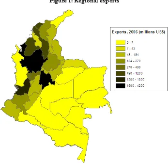
The objectives of this study are to quantify the extent to which domestic transport costs act as a friction for the international trade of goods and to examine how improvements in road quality impact trade performance. We employ a methodology that combines real freight costs and Geographic Information System (GIS) analysis to obtain a realistic measure of the domestic transport costs. The methodology is applied to the case of Colombia, a developing country with significant regional disparities in terms of trade performance (see Figure 1). The analysis consists on estimating a model in which regional exports depend on the freight costs of shipping the exports from their location of production to their ports of shipment (ports, airports or borders) controlling for several other factors. The model is then used to predict how changes in road quality affect export performance. Our study is somewhat related to Albarran, Carrasco and Holl (2009) which also uses GIS analysis to examine how transport network improvements affect the likelihood of exporting among Spanish firms. One of the main differences with our study, however, is the measure of transport costs. While these authors use travel time to proxy for transport costs, we significantly improve this measure by explicitly estimating the transport costs associated with travel time and also with distance. This is important because the effects of improvements in the transport network are not limited to time-related costs but are also associated with distance-related costs, as we will show in the analysis.
times more than regions with transport costs in the 75th percentile, once other factors are controlled
for. An improvement in road quality that generates an average reduction in transport costs of 12% increases average exports by around 9%. The gains are found to be larger in regions with initially higher transport costs. This is because regions with initially higher transport costs are normally associated with longer routes and those tend to have larger shares of roads in poor conditions.
The next section explains the estimating methodology which takes in consideration key insights from various economic geography and trade models. Section III describes the construction of the different datasets and section IV presents the results. Some concluding remarks are presented in section V.
II. Methodology
The point of departure of our model is a simple log-linear relationship between regional exports and domestic transport costs:
jrpt jrpt
jrpt tc
E =β0 +β1⋅ +μ (1)
where Ejrpt is the (log of) exports of good j from region r to port p in year t 1,
jrpt
tc is the (log of) ad-valorem transport costs of shipping good j from region r to port p in year t, and μjrpt is the error
term. A chief econometric concern with this equation, however, is the potentially large number of omitted variables that could bias the econometric results. For instance, there might be several factors leading to the initial agglomeration of firms in a particular region and consequentially inducing a large level of exports from this place. Regressing regional exports on a measure of domestic transport costs without controlling for these factors is likely to produce biased results. In what follow we rely on key elements of the economic geography literature to address this issue.
One insight from economic geography models is the notion that plant-level scale economies interacted with transport cost leads to the agglomeration of firms in the large market. Sometimes referred as the home-market effect, firms tend to locate in the large market because they will be able
to enjoy larger profits derived from lower transport costs and from a drop in their average production costs. A second set of factors that could lead to agglomeration has to do with the presence of externalities. To the extent that externalities are localized, economic activity tend become geographically concentrated over time. Empirical support to this idea has been found, for example, in Glaeser et al. (1992), Jaffe et al. (1993) and Henderson et al. (1995). A third factor is related to the presence of backward-forward linkages. The original Hirschman’s (Hirschman, 1958) concept that vertical relationships between industries create a pattern of interdependent industry location has been formalized many times in the literature (e.g. Venables, 1996; Krugman and Venables, 1995). Other factors attracting firms to particular locations are known under the general heading of natural amenities and local public goods (Combes, Mayer and Thisse, 2008). These factors can range from natural endowments (like the presence of lakes or rivers) to public services (like schools, hospitals or telecommunication infrastructure).
Several proxies have been used in the economic geography literature to estimate the effects of these forces on outcomes like regional wages. For instance, a density measure consisting on the employed in the region divided by its surface area is frequently used to capture the home-market effect. Various indexes of regional diversification have been employed to capture the effects of inter-industry externalities. Measures of endowments, like arable land, or several classes of public investments are also normally used to account for the presence of natural endowments and/or the existence of public goods. The list of factors can be quite large and normally varies depending on the focus of the investigation with variables like regional GDP, the average skilled level of the population or the number of firms in the region being a few more examples.
Besides the region-year fixed effects, we employ additional dummy variables to control for additional elements. For instance, while our focus is on the trade impacts of domestic transport cost, neglecting the existence of international freights may introduce some biases. A simple example can illustrate the point: some ports in Colombia are located in the Pacific side of the country while others are in the Atlantic side. A firm located near the Pacific side and seeking to export to the east coast of the United States might ship by land most of its goods to a port on the Atlantic side. By doing this, the firm might pay higher domestic transport costs than shipping the goods to a port in the Pacific side, but at the same time, it might reduce the overall transport costs of the entire shipment (domestic plus international freights) by paying lower international freights. Therefore, for this firm, large volumes of exports will be associated with large domestic freight rates and low volumes of exports will be associated with small domestic freights. It is clear that not controlling for the international component of the transport costs might bias the econometric results. Unfortunately, we do not have an adequate dataset for the international transport cost of the Colombian exports. However, given that the relative distances between the Colombian ports and the destination markets are fixed, we can capture this aspect using port dummies. Specifically, we add port-commodity-year dummies to account for the possibility that these relative costs are commodity-specific and that they vary over time.
Note that having introduced commodity and year dummies also control for commodity-specific characteristics like the tradability of the good or for country-wide-time-variant factors like exchange rate shocks. Equation (1) then changes to:
jrpt t
j p t r jrpt
jrpt tc
E =β1⋅ +α ⋅α +α ⋅α ⋅α ++μ (2)
where, αr, αt, αp and αj are fixed effects for region, year, port and commodity, respectively. This
III. Construction of Datasets
III.A. Transport Costs
We combine spatially geo-referenced data of the Colombian road network with truck operating costs in the country to obtain a realistic measure of the domestic transport costs. The measure is the cost for a reference truck to ship one ton of cargo through the cheapest route that connects any pair of locations. In essence, this measure is a very close approximation of the shipping cost incurred by carriers when using the actual transport network of the country assuming that they select the minimum cost route between any two locations.2 The cost estimation is based on a methodology described in Combes and Lafourcade (2005). Here, we summarize the key insights of this methodology.
The transport network of a country consists on a number of arcs of different types (e.g. highways, primary roads, secondary roads, etc). Along any particular arc, there are two types of costs: costs associated with distance and costs associated with time. The distance-related costs per km are essentially fuel costs, tire renewing expenses and maintenance operating costs. The time-related costs per hour are the labor costs, the insurance expenses, the depreciation costs, as well as carrier vehicle taxes and parking costs.
Let da denote the distance between the end-nodes of an arc a; then, the total
distance-related costs incurred when connecting two locations r and p at date t using a route Zrpt is given by:
(
)
∑
∈ ⋅ + + = rpt Z a a t t trpt fuel tire main d
C
Dist_ (2)
Similarly, let sa be the speed along the arc a, then the time for joining the arc nodes is
a a a
s d
t = , and the total time-related costs incurred when connecting two locations r and p at date t
(
)
⎟⎟ ⎠ ⎞ ⎜ ⎜ ⎝ ⎛ ⋅ + + + + =∑
∈Zrpt
a a a t t t t t rpt s d parking taxes deprec insure wage C
Time_ (3)
Obviously, there could be many different routes joining locations r and p, but we are interested in the route with the lowest total costs. Therefore, if ωrpt denotes the set of all possible routes that join
locations r and p, the optimization problem for finding the route with the minimum transport costs (Total_Crpt) is:
) _ _
( min
_ rpt rpt
Z
rpt Dist C Time C
C Total rpt rpt + = ∈ω (4)
This optimization problem is solved using geographic information system (GIS) software (ArcView) and a digitalized transport network of Colombia. The network is populated using real distance and time-related costs data taken from the Colombian Ministry of Transportation which, in turned, are gathered from transportation surveys conducted by the Ministry. These costs vary by class of truck and year. The class of truck chosen for this study corresponds to the most popular truck configuration used in the country. 3
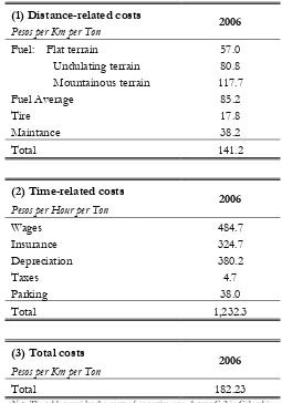
Table 1 presents a summary of the average distance and time related costs for the year 2006. Fuel expenses are differentiated by type of terrain, and on average they represent the most significant distance-related cost while wages as well as depreciation costs account for the most significant time-related costs. Panel (3) of the table calculates the total reference cost per ton per km which is obtained by adding the total distance-related costs and the total-time related costs once the latter is divided by the average speed of the class-truck selected in the country. 4
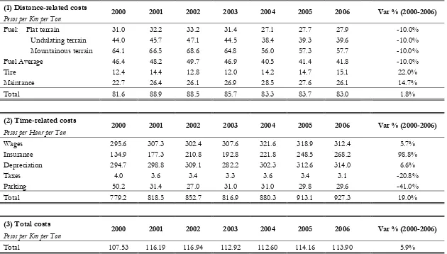
While we are mostly interested in exploiting the cross-regional variation of the data, the time-series dimension of the transport costs could also be relevant. Table 2 shows the costs between 2000 and 2006 in constant terms and provide information about the deflators used. In real terms the
2 Note that this cost estimate does not include any potential markup charged by transport companies.
total costs increased by around 6%, however, some of the costs increased much more, like the tire costs (on the distance-related costs) and insurance (on the time-related costs).
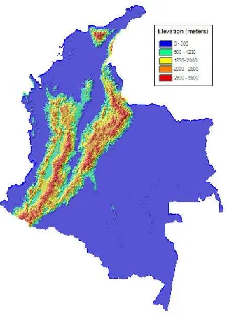
Our estimation of the transport costs takes into consideration the type of surface traversing the road network. According to the Ministry of Transportation, the fuel consumption of the class truck selected varies by the type of surface (see Tables 1 and 2). Adjusting transport costs to the type of surface traversing the roadways is important particularly for a country like Colombia with a considerable area covered by mountainous terrain (see Figure 2). In order to account for type of terrain we first convert the geo-referenced surface layer of Colombia, shown in Figure 2, from elevations into slopes. Then, merging the slope layer with the road network layer we identify for each segment of every road in the network, its average slope. According to the Ministry, slopes below 3 degrees correspond to flat terrain, between 3 and 6 degrees correspond to undulating terrain and above 6 degrees correspond to mountainous terrain. Therefore, fuel consumption is adjusted according to these three types of slopes using the values provided in Table 2.
III.B. Adjustment for Road Quality
To account for the effect of the quality of the road network on transport costs, we are required to obtain information about the conditions of the roadways in Colombia as well as information on how these conditions affect the various costs of operating a truck in the country. It is worth starting with a brief discussion on measuring road quality.
The IRI is based on the average rectified slope which is a filtered ratio of a standard vehicle’s accumulated suspension motion (in millimeters) divided by the distance traveled by the vehicle during the measurement (meters). Therefore, the IRI is commonly expressed in millimeters per meter (mm/m) or in meters per kilometer (m/km).
While the IRI has an open-ended scale, it typically ranges from 0 (mm/m) to 20 (mm/m) where zero implies an absolute perfection of the road. Normally, the IRI is related to road quality in the following way: below 1.7 for airport runways and superhighways; 1.7-3 for new payments and older payments in good conditions; 3-9 for roads with surface imperfections, including some older payments, some damaged pavements and some maintained unpaved roads; 9-14 for roads with frequent shallow depressions that in some cases could be deep, including some damaged pavements, some maintained unpaved roads and some rough unpaved roads, and more than 14 associated with unpaved roads in erosion gullies or deep depressions. For a detailed discussion on the IRI, see UMTRI, 2002.
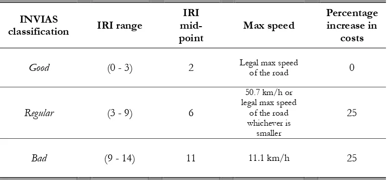
The Colombian national road authority, Instituto Nacional de Vías (INVIAS), keeps track of the conditions of the primary roads in the country. The Institute divides the conditions of each arc in the primary road network in broad categories as “good”, “regular” and “bad”. To measure the conditions of the roads, INVIAS employs a visual inspection to provide a general assessment of the traversability condition of the road. Based on measurement guides from INVIAS, the broad categories used by the institute can roughly be matched with the IRI in the following way: good (0-3), regular (3-9) and bad (9-14), where the numbers in the parentheses correspond to the IRI.
III.C. Geographical Scale and Trade Data
We work at the municipality level using the 1,111 municipalities identified in the 2005 economic census (carried by DANE). We exclude two dozen municipalities (like San Andrés and Providencia islands) because either we do not have information on their road networks or because they are not physically connected with the rest of the country with roads in the primary, secondary or tertiary networks (like some municipalities in the Amazonas Department). For each municipality we calculate its centroid consisting on the weighted average of all the x’s and y’s coordinates of the perimeter of the municipality. The centroid is where we locate geographically the origin of the exports for each municipality.
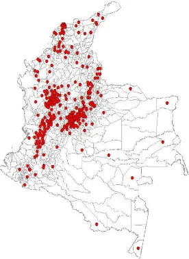
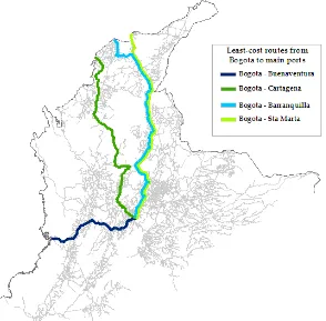
The regional exports at the product level (10 digit HS) includes information of the municipality of origin and the custom through which the merchandise exits the country. Therefore, for each export, we have a record of the origin of the shipment and the custom destination used to exit the country. These trade data come from Dirección de Impuestos y Aduanas Nacionales (DIAN). It is worth mentioning that the majority of the municipalities do not export (see figure 3). Only 27% of all municipalities export a good in the period of the study. This issue will become relevant in the next section when we discuss potential econometric biases in the estimation. Regarding the customs, there were a total of 20 active customs during the period of consideration. These customs are distributed across the country in various ports, airports and land borders and were located in the transport network using their precise addresses. The 1,111 origins and the 20 destinations comprise a total of 22,220 potential routes. Figure 4 illustrates, geographically, an example of the outcome from the optimization process. It depicts the least-cost routes from one origin, Bogota D.C., to four custom destinations: Barranquilla, Buenaventura, Cartagena, and Santa Marta ports.
Once we obtained the transport costs of shipping 1 ton of generic merchandise along these routes using equation (4), we then calculate the ad valorem transport costs for each product used in equation (2) as follows:
jrpt jrpt rpt jrpt
E w C Total
where wjrpt is the weight (expressed in tons) of good j that is transported from region r to port p in
year t, and Ejrptis its export value as defined before.
One potential bias generated by the methodology used to construct the transport costs in this study is related to the selection of the least-cost route as the route that defines the transport costs between any two locations. If shipping companies deviate largely from the least-cost route, then the transport costs that they face might differ from the ones estimated in this study. Note that in principle the least-cost route is not an unrealistic assumption, profit maximizing shipping companies have the incentives to select the cheapest route between any two locations. However, there might be factors outside their control that preclude them to do so (i.e. certain road restrictions, lack of security in particular roads, etc).
We performed a simple exercise to evaluate whether this should be a source of concern. In Colombia, the minimum freight value that a registered transport company must pay to the owner of a vehicle is regulated by the Ministry of Transportation. This value is updated every year and is published in a matrix of origins and destinations comprising a total of 18 origins and 22 destinations (for the year 2008). The freight values are related to calculations about transport costs made by the Ministry of Transportation using the same surveys that we employed regarding the operating costs of trucks in the country. While the methodology used by the Ministry is similar to the one in this study, in the sense that they calculate the total cost of a route that combines distance and time related costs, the Ministry does not use an optimization process to select the least-cost route. The information about the routes between locations is based on the most commonly used routes by transport companies gathered also from surveys. With this information, they estimate the transport costs across all pair of origins-destinations they have selected.5 In order to validate the methodology
that we employed in this study, we estimated the transport costs for the same group of cities and compared them with the estimates of the Ministry. The correlation between the two estimations (across all the pairs of cities) is equal to 0.93 and significant at the 1% level. Therefore, as the two estimations do not deviate in any considerable way, the selection of the least-cost route as the route that defines the transport costs between any two locations should not be a reason of concern.
Another potential econometric concern is related to the existence of modes of transportation different than roads. If certain activities employ alternative modes of transportation, the costs of shipping - and consequentially the trade effects of transport costs - are not necessarily bounded by the road network of the country. Not accounting for these alternative modes of transportation could generate biased econometric results. In Colombia, however, most of the cargo within the country is carried by trucks. According to the Ministry of Transportation, for example, around 95% of all non-coal cargo (in tons) is transported by trucks and the rest 5% is divided across rail, air and the fluvial modes. This implies that no significant biases should be expected by focusing on road-related transport costs. Having said this, it is worth noting that within some sectors it is well-known that the main mode of transportation is not the truck. These sectors are essentially mining and the oil industry which use other means of transportation extensively. For instance, coal is transported within Colombia primarily through the rail system while oil is transported mainly through pipelines. Therefore, the transport costs in these industries are not necessarily referenced by the road-related transport costs estimated in this analysis. To avoid generating bias results from these industries, we exclude them from the econometric estimation.
IV. Econometric Results
IV.A. Initial Estimation and Robustness Tests
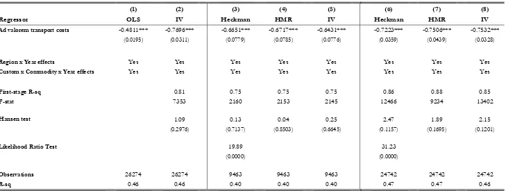
The empirical strategy consists on an eclectic econometric approach in which we apply a variety of estimation techniques recently proposed in the literature to control for many potential biases in measuring the impact of trade barriers. The estimations are for the period 2004-2006 and are carried at the 4 digit ISIC (rev3) level. Column (1) in table 4 presents the initial outcome when the regression is estimated using OLS together with the fixed effects. The results show that domestic transport costs are negatively and significantly related to regional exports with an elasticity of 0.48. In other words, a reduction of transport costs in 10% increases regional exports in about 4.8%.
employ an instrumental variable estimation (IV). Our first instrument is the total distance of the route. We argue that distance affects regional exports only through its impact on the costs of transportation; therefore, the necessary condition of a zero correlation between the instrument and the error term in equation (2) is likely to be met. Our second instrument is the length of the route on mountainous and undulating terrain. As we mentioned before, the type of terrain also affect the cost of transportation beyond the impact of distance per se and its impact on regional exports should be precisely through this effect. In order to examine the validity of these variables as exogenous instruments, we perform tests of overidentifying restrictions.
The results, shown in column (2), indicate that controlling for the potential endogeneity does not affect the significance of the coefficient. Indeed, the export elasticity increases in absolute value to 0.77, meaning that a reduction of transport costs in 10 percent increases regional exports in about 7.7 percent. The coefficient estimate for this model implies that regions with transport costs in the 25th percentile export around 2.3 times more than regions with transport costs in the 75th percentile,
once the other factors are controlled for. The R-square of the first stage regression is considerably large as well as the F-statistic for the join significance of the instruments indicating that we do not have a weak-instrument problem. Additionally, the Hansen test of overidentifying restrictions shows that we cannot reject the null hypothesis that the instruments are valid.
A potentially different econometric problem is related to the sample used in the estimation. Our data only include the exports that are recorded, in other words, the exports with positive values. Therefore, a potential problem is related to the notion that the sample we are using is not representative of the population. As we point out before, there are many municipalities that do not export any good. However, it is possible that many of them produce goods for the domestic market. By not including these zero-value-exports in the estimation our sample is technically censored which may lead to inconsistent parameter estimates. Moreover, as the observations in the sample are not randomly selected (only the exports with positive values are included in the sample) the results may suffer from selection bias. To address these potential econometric problems we estimate a Heckman selection model.
from the General Census of 2005 (conducted by Departamento Administrativo Nacional de Estadística, DANE). The census provides information about the number of establishments that were active in each municipality at the 4 digit ISIC (rev 3) industry level. This is the same level of disaggregation used in the previous estimations.The merge then allows us to assign zero-value exports to those municipalities that produced goods but did not export them. 6
The second step to estimate the Heckman model is to add the transport costs associated with these zero-value observations. This requires making two assumptions. The first assumption is related to the port of shipment. Since we do not observe the export, we do not know from which port the output would have been shipped out of the country. This implies that we do not have a route in order to assign a transport cost. To address this issue we make the conservative assumption that the good would have been shipped from the municipality of origin to the port in the country that gives the cheapest route. The second assumption has to do with the weight-to-value ratio employed in the calculation of the ad valorem transport costs (see equation 5). Since we do not observe the export value or its weight, we do not have the second term in equation 5 which is necessary to estimate the ad valorem transport costs. However, weight-to-value ratios are mainly determined by factors not necessarily associated with location: the weight is an intrinsic characteristic of the commodity and its export value is, for the most part, determined by international prices. Therefore, the weight-to-value ratio used in the calculation of the ad valorem transport costs for any good produced and not exported is the average weight-to-value ratio of all the exports of that good with positive values. For the cases in which the good was never exported, the weight-to-value ratio is the average weight-to-value ratio of the exports of the immediate more aggregated level of classification (1 digit less).7
The third step for estimating the Heckman model is to choose a valid exclusion restriction in the selection equation. This is a delicate task as the exclusion restriction should generate nontrivial variation in the selection variable but should not affect the outcome variable directly. To choose our exclusion restriction we rely on empirical evidence and theoretical background. There is a large body of empirical evidence showing that exporting firms tend to be larger, more productive and more capital intensive that their non-exporting counterparts. A common argument explaining this
evidence is that only the more productive firms can pay for the high sunk costs of exporting; therefore, firms self-select into export markets. Indeed this is one of the core assumptions in recent influential theoretical trade models with heterogeneous firms (Melitz, 2003 and Bernard et al., 2003). Evidence of self-selection have been found in Bernard and Jensen (1999), Clerides, Lach and Tybout (1998), Aw, Chung and Robert (2000). These authors show that plant productivity increases before entry to export markets, but does not change, or changes very little, after entry. Therefore, there is strong evidence of self-selection and only weak support for what is called the learning-by-exporting hypothesis. 8
Based on this theoretical and empirical background we choose the average size of all the firms producing good j in region r, as our exclusion restriction. The argument is that only the plants that become sufficiently productive (large) enter the export market but after entry the productivity of these exporting plant changes very little, if at all. Therefore, the variable should satisfy the exclusion restriction requirements, namely that it is a relevant factor in the selection equation but that it can be reasonably excluded from the outcome equation. The variable is constructed as the average size, in terms of number of employees, of all the firms in the 4-digit ISIC (rev 3) industry in each municipality. The number of employees per firm is taken from the General Census conducted by DANE.
The production data (that is, the number of active firms and the average size of the firm) are available only for the industry sector. Therefore, we focus the estimation of the Heckman model to the industry sector. The results are shown in column (3) which also controls for the reverse causality mentioned before: that is, we estimate the selection equation, calculate the inverse mills ratio, and use it in the outcome equation while instrumenting for the transport costs using the same instruments as before. Note that the sample size dropped significantly. This is because in many cases the variables in the model, including the sets of fixed effects, predict success or failure perfectly in the selection equation making the probit model to drop the associated observations. Later we estimate an alternative version of the Heckman model with a less stringent set of fixed effects.
7 For instance, if sub-category 1511 (from ISIC rev3) was never exported, we assume its weight-to-value ratio is given by the average of the exports in the 151 sub-category.
The results suggest the existence of selection: the likelihood ratio test for the independence between the selection and the outcome equations is rejected in favor of using the Heckman selection model. More importantly, the coefficient for the transport costs continues to be negative and significant after correcting for the sample selection bias. In column (4) we also run the well-known Helpman-Melitz-Rubinstein (HMR) procedure which simultaneously corrects for sample selection and firm heterogeneity biases.9 The result show that the coefficient for the transport costs continues
to be negative and significant with an elasticity of -0.67.
Note that the elasticities in columns (3) and (4) are somewhat lower than in column (2). Therefore, in column (5) we repeat the IV estimation using the same sample as in the Heckman and HMR estimations. The elasticity is -0.64 which is very similar to the elasticity in the Heckman and the HRM estimations. This shows that the differences in the elasticity between column (2) and the Heckman and HRM estimations (columns 3 and 4 respectively) are mainly due to the change in the sample size rather than the result of correcting for the sample selection or the firm heterogeneity bias.
We now estimate a variation of the Heckman and HRM models using a more parsimonious set of fixed effects in the selection equation. Specifically we use only region fixed effects in the selection equation but keep the full set of fixed effects in the outcome equation. This allows us to estimate the selection equation more freely. In other words, this reduces the cases in which the variables of the model completely determine success or failure, reducing the number of observations that are dropped in the probit regression. The results (column 6 and 7) are once again compared to an IV estimation (column 8) using the same sample of observations. The coefficient for the ad valorem transport cost in the Heckman and HRM models continue to be negative and statistically significant. Note that once again the elasticities are not very different from the one obtained in the IV estimation.10
9 See Helpman, Melitz and Rubinstein (2008) for details.
10 Helpman, Melitz and Rubinstein (2008) show that controlling for selection normally leads to a reduction in the estimate of the trade barrier coefficient (becomes larger in absolute value) while controlling for firm heterogeneity normally leads to an increase in the coefficient (becomes smaller in absolute value). We do not observe such a pattern in our regressions because the regressor, the ad valorem transport costs, is instrumented by different variables in each model. For instance, in the model based only on IV, the instruments for transport costs are the total distance of the route and the length of the route on mountainous and undulating terrains, as mentioned before. In the Heckman model, however, the instruments include these two variables but also the inverse mills ratio. In the HRM, the instrument list also includes the correction for the firm heterogeneity. As such, the
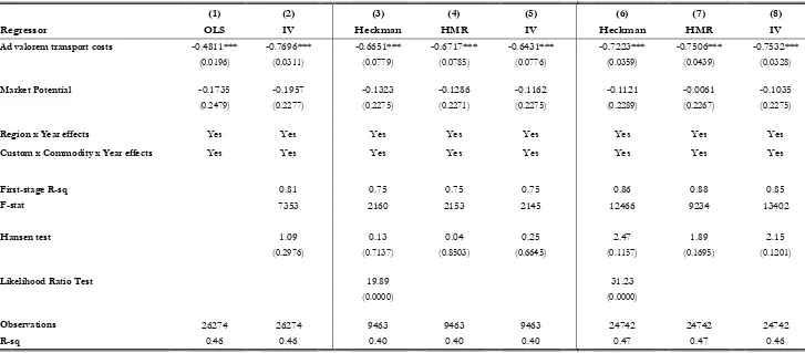
Before moving into the next section, there is another potential bias related to the fact that we are using spatially-related data. So far, the implicit assumption has been that there are no interactions between regions. However, it could be the case that firms in one region might benefit from neighboring regions. For instance, one municipality might benefit from interindustry or intraindustry externalities emanating from other municipalities. Not taking into consideration these interactions is equivalent of having an omitted variables problem which could bias the econometric results. One way to address this concern is to employ techniques from spatial econometrics. For example, we could add spatially lagged variables to account for potential autocorrelation of the residuals (see Anselin et al, 2003). Using spatial econometrics while correcting for reverse causality and addressing the zero-value observations bias at the same time proves to be a challenging exercise. Our preferred strategy is to borrow a standard practice in the economic geography literature for dealing with this issue which consists on adding a market potential variable into the estimation. The idea goes back to Harris’s (1954) who defined the market potential of a region as the sum of all the other region’s densities weighted by the inverse of their distance to this region. The notion is that this variable will capture any bias resulting from spatial dependence. We improve the construction of the market potential variable by employing the real transport costs between regions instead of distance. These transport costs are calculated as in equation (4). Table 5 shows the results of estimating all the models in table 4 after including the market potential as an additional covariate. The coefficients for the market potential turned out to be not significantly different from zero. More importantly, the coefficients for the ad valorem transport costs do not change in any significant way.
IV.B. Simulation: Improvement in Road Quality
In this section we simulate what would be the effect on regional exports of a reduction in transport costs generated by improvements in road quality. Specifically, we simulate the reduction in transport costs that would arise if the conditions of all the roads identified as “bad” and “regular” by INVIAS improve to good. It is worth mentioning that in 2005, the year that we used for the information on road conditions, 47% of the primary road network (under the jurisdiction of INVIAS) was in good condition, 33% in regular condition and 20% in bad condition.
It is worth remembering that improving the condition of a road reduces the costs of transportation through two effects: first, it increases the speed by which the road can be traversed and consequentially, it reduces all the costs that are associated with time (see equation 3). Second, it lowers the maintenance, repair, tire and depreciation costs associated with using that road.
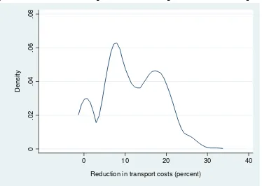
The reductions in transport costs generated by the improvement in road quality vary greatly depending on the route. For instance, while the average reduction in transport cost for all the routes is equal to 11.6% the standard deviation is 7%. This is because some routes have large shares of roads in regular and bad conditions while others are in good conditions for the most part. The large standard deviation implies that there are several routes with declines in transport costs below 5% but also many routes with declines in transport costs above 15%. Indeed, we observe several routes with reductions in transport costs as high as 30%. Figure 5 shows the distribution of the reductions in transport costs for all the routes.
It is also important to mention that the correlation between the decline in transport costs and the initial level of transport cost is positive (0.51) and significant at the 1% level. In other words, routes with initially higher levels of transport costs tend to exhibit larger declines. This is explained because the regions with initially higher transport costs are mostly associated with longer routes and longer routes tend to have larger shares of roads in poor conditions, as shown in Figure 6.
networks of the country even though they are used –together with the primary road network- to select the least-cost routes. For all the roads on the secondary and tertiary networks we have made the conservative assumption that they are all in good conditions. Second, the primary road network with information about road quality is limited to the roads under the jurisdiction of INVIAS, the public entity in charge of the roadways. This excludes the roads under concessions contracts with the private sector. Roads under concession contracts in the primary network represent 17% of all the roads. Once again, we have made the conservative assumption that all these roads are in good conditions.
To perform the simulation we used the econometric estimates from column (2) in Table 4. Since the export elasticity of transport costs does not vary much after correcting for sample selection or firms heterogeneity bias, this model also allows us to predict the export response in the agricultural, forestry and fishing sectors besides the industry sector. Alternative simulations performed with the estimations form the Heckman and HMT models provide similar qualitative results.
The simulated reduction in domestic transport costs induces an average increase of export of 9% with a standard deviation of 6%. The gains are found to be generally larger in the regions with the initially higher transport costs, as shown in Figure 7. For instance, the average increase of export in regions with initial transport costs below or equal to the 25th percentile is 4% while the average
increase of exports in regions with transport costs in the 75th percentile or above is 11%. This is mostly explained by what we mentioned before: the routes with the highest transport costs tend to be the longest routes, and those normally have larger shares of roads in regular and bad conditions. The result implies that the improvement in road conditions tend to favor relatively more the export performance of the more remote regions.
V. Concluding Remarks
extent to which domestic transport costs act as a friction to international trade. We find an export-elasticity to domestic transport cost in the order of 0.75. This implies, for example, that regions with transport costs in the 25th percentile export around 2.3 times more than regions with transport costs
in the 75th percentile, once other factors are controlled for.
References
Ahlin, K. and J. Granlund. 2002. “Relating Road Roughness and Vehicle Speeds to Human Whole Body Vibration and Exposure Limits” The International Journal of Pavement Engineering. Vol 3(4)
Albarran, P., R. Carrasco and A. Holl. 2009. “Transport Infrastructure, Sunk Costs and Firm’s Export Behavior” Working Paper 09-22. Universidad Carlos III de Madrid.
Alvarez, Roberto, and Ricardo López. 2005. “Exporting and Performance: Evidence from Chilean Plants”. Canadian Journal of Economics. Vol 38, No.4: 1385-1400.
Anselin, L., R. Florax, and S. Rey. 2003. Advances in Spatial Econometrics. Springer
Aw, B., S., Chung, and M. Roberts (2000). “Productivity and turnover in the export market: micro-level evidence from the Republic of Korea and Taiwan (China), World Bank Economic Review, 14, 65-90
Barnes, G. and P. Langworthy. 2003. “The Per-Mile Costs of Operating Automobiles and Trucks” Report No. MN/RC 2003-19. Published by Minnesota Department of Transportation
Benedictis, G., G. Calfat and R. Flores Jr. 2006. “Challenging the pro-development role of trade agreements when remoteness counts: the Ecuadorian experience” Working Paper 2006.5, University of Antwerp.
Bernard, Andrew, Jonathan Eaton, Bradford Jensen and Samuel Kortum. 2003. “Plants and Productivity in International Trade”. American Economic Review. Vol 93, No 4: 1268-1290.
Clark, Ximena, David Dollar and Alejandro Micco. 2004. “Port Efficiency, Maritime Transport Costs, and Bilateral Trade”. Journal of Development Economics. Vol 75: 417-450.
Clerides, S., S. Lach, and J. Tybout (1998). “Is Learning by Exporting Important? Micro-dynamic Evidence from Colombia, Mexico and Morocco”, Quarterly Journal of Economics, 113.
Combes, P.-P., and M. Lafourcade. 2005. Transport Costs: Measures, Determinants, and Regional Policy. Implications for France. Journal of Economic Geography. 5.
Combes, P.-P., T. Mayer and J.-F. Thisse. 2008. Economic Geography, the Integration of Regions and Nations. Princeton University Press.
Costa-Campi, M. T. and M. Viladecans-Marsal. 1999. “The District Effect and the Competitiveness of Manufacturing Companies in Local Productive Systems”. Urban Studies. 36.
Glaeser, E. L., H. Kallal, J. Sheinkman, and A. Schleifer. 1992. “Growth in Cities”. Journal of Political Economy. 100.
Harris, C. 1954. “The Market as a Factor in the Localization of Industry in the United States”.
Annals of the Association of American Geographers. 64
Henderson, J. V., A. Kuncoro, and M. Turner. 1995. “Industrial Development in Cities”. Journal of Political Economy. 103.
Hirschman, A.O. 1958. The Strategy of Economic Development. Yale University Press, New Haven.
Hummels, David. 2001. “Toward a Geography of Trade Costs”. Department of Agricultural Economics, Purdue University. Mimeographed document.
Hummels, David & Lugovskyy, Volodymyr & Skiba, Alexandre. 2009. “The Trade Reducing Effects of Market Power in International Shipping”. Journal of Development Economics. Vol 89, No 1: 84-97
Jaffe, A., M. Trajtenberg, and R. Henderson. 1993. “Geographic Location of Knowledge Spillovers and Evidenced by Patent Citations” Quarterly Journal of Economics. 108.
Krugman, P., and A.J. Venables. 1995. “Globalization and the Inequality of Nations”. Quarterly Journal of Economics. 110.
Lafourcade, M., and E. Paluzie, 2008. “European Integration, FDI and the Geography of French Trade” Regional Studies (forthcoming).
Matthee, M., and W. Naudé. 2007. “The Determinants of Regional Manufactured Exports from a Developing Country”. Research Paper No. 2007/10. UNU-WIDER World Institute for Development Reconomics Research.
Melitz, Marc J. 2003. “The impact of trade on intra-industry reallocations and aggregate industry productivity” Econometrica. Vol 71, No 6: 1695-1725
Micco, Alejandro, and Tomas Serebrisky. 2006. “Competition Regimes and Air Transport Costs: The Effects of Open Skies Agreements”. Journal of International Economics. Vol 70 (1): 25-51
Moreira Mesquita, Mauricio, Christian Volpe and Juan Blyde. 2008 Unclogging the Arteries: The Impact of Transport Costs on Latin American and Caribbean Trade, Special Report on Integration and Trade. Washington, DC, United States: Inter-American Development Bank.
Nicolini, R. 2003. “On the Determinants of Regional Trade Flows” International Regional Science Review. 26(4)
Silva, J.M.C. and S. Tenreyro (2006). “The Log of Gravity” The Review of Economics and Statistics, Vol. 88, No. 4: 641-658.
UMTRI. 2002 University of Michigan Transportation Research Institute, Research Review, Volume 33, Number 1.
Venables, A.J. 1996. “Equilibrium Locations of Vertically-linked Industries” International Economic Review. 37.
Appendix I
Adjustment of transport costs to road quality
I.A. Adjustment of speed
The first adjustment that we make is related to vehicle speed. It is natural to think that vehicle speed is negatively associated with the roughness of roads, but in the absence of speed measurements taken directly on the roadways, it is difficult to assess how much drivers would slow down when the conditions of the roads deteriorate. One way to go about this is to assess how road quality determines the quality of the ride. In this area there are several international guidelines developed for health-related reasons. For example, ISO 2631-1 defines how to quantify human whole-body vibration (WBV) experienced by the driver and passengers during the ride, in relation to health and comfort. These guidelines have been used, for instance, to derive maximum speed limits. One interesting application of these guidelines is carried by Ahlin and Granlund (2002). The authors estimate a relationship between road roughness (measured in terms of the IRI), vertical human WBV and vehicle speed and combine it with ISO guidelines to convert limits for WBV to corresponding approximate limits for IRI and/or vehicle speeds.
Starting with the quantification of human WBV, this measurement is normally expressed in terms of the frequency-weighted acceleration at the seat of a seated person or the feet of a standing person and can be measured in units of meters per second squared (m/s²). According to ISO 2631, the base reaction level for WBV is called “not uncomfortable”, and goes from zero (0 m/s2) up to 0.315
m/s2. Over that level, the reaction is expected to be “a little uncomfortable”. When the exposure
exceeds 0.5 m/s2, the reaction is expected to be “fairly uncomfortable”. This level, for example,
Ahlin and Granlund (2002) use these guidelines in their calculation. Essentially they employ a mathematical model to first derive a relationship between road roughness, vertical human WBV and vehicle speed. Then, using the 0.8 m/s2 as the limit for the WBV, corresponding to “uncomfortable”
according to ISO 2631, they derive the following relation between “comfortable vehicle speed”, cvs [km/h], and IRI [mm/m]:
n IRI
cvs ⎟−
⎠ ⎞ ⎜ ⎝ ⎛ ⋅ = 1 2 5 80
where n is a parameter for the amplitude of the roughness 11. For most of the roads, the exponent
n
has a value around 1.8. Therefore, for a road with roughness equal to 6 in terms of IRI, the comfortable vehicle speed should be below 50.7 km/h. At speeds above this value, the ride would be “uncomfortable” according to ISO 2631 and may have long term health consequences to the driver. We use this formula to derive driving speeds in the arcs in the Colombian network according to their conditions. Table 3 presents the relationship between road condition, IRI and the resulting speeds that we use (column 4).
I.B. Adjustment of maintenance, repair, tire and depreciation costs to road quality
While lower speeds affect transport costs of any route through the time-related costs portion of these costs, another way transport costs are affected by the quality of the road network is by the direct impact on charges that vary in direct proportion of the roadway conditions. Typically these charges are related to maintenance, tire, repair and depreciation costs. The latter is related to the reduced vehicle life.12 Following this, Barnes and Langworthy (2003) presents a mathematical model
for highway planning that calculates the costs of operating cars and trucks and also incorporates adjustments factors according to roadway conditions. The authors based their adjustment multipliers on available empirical assessments from various countries, including the US and New Zealand.
11 The value of n is low for roads where the dominating roughness amplitudes have short wavelengths, such as on a modern designed highway with a deteriorated surface with plenty of potholes. The value of n is high for roads where the dominating roughness amplitudes have long wavelengths, such as on an ancient designed rural low volume road (Ahlin and Granlund, 2002).
According to the authors, the adjustment multiplier for maintenance, repair, tire and depreciation costs for an IRI equal or higher than 2.7 is, 1.25. In other words, maintenance, repair, tire and depreciation costs increase by 25% when the truck transits road with conditions associated with an IRI’s equal or greater than 2.7. We take this study as a general guide on how to increase maintenance, repair, tire and depreciation costs in our calculations. Table 3 (column 5) presents the information. Essentially we increase these costs by 25% when the road is classified as “regular” and also when the road is classified as “bad”. 13
Table 1: Operational Transport Costs
(1) Distance-related costs
2006
Pesos per Km per Ton
Fuel: Flat terrain 57.0 Undulating terrain 80.8 Mountainous terrain 117.7
Fuel Average 85.2
Tire 17.8 Maintance 38.2 Total 141.2
(2) Time-related costs
2006
Pesos per Hour per Ton
Wages 484.7 Insurance 324.7 Depreciation 380.2 Taxes 4.7 Parking 38.0 Total 1,232.3
(3) Total costs
2006
Pesos per Km per Ton
Total 182.23
Note: The table provides the costs of operating a truck type C-2 in Colombia according to cost figures given by the Minister of Transportation. Total costs = (distance_related costs ) + ( time_related costs/average speed) .
Source: Authors calculation based on data from the Ministry of Transportation, Colombia
Table 2: Operational Transport Costs in Constant Values (base year=2000)
(1) Distance-related costs
2000 2001 2002 2003 2004 2005 2006 Var % (2000-2006)
Pesos per Km per Ton
Fuel: Flat terrain 31.0 32.2 33.2 31.4 27.1 27.7 27.9 -10.0% Undulating terrain 44.0 45.7 47.1 44.5 38.4 39.3 39.6 -10.0% Mountainous terrain 64.1 66.5 68.6 64.8 56.0 57.3 57.7 -10.0%
Fuel Average 46.4 48.2 49.7 46.9 40.5 41.4 41.8 -10.0%
Tire 12.4 14.4 12.8 12.0 14.2 14.7 15.1 22.0%
Maintance 22.7 26.4 26.1 26.9 28.5 27.6 26.1 14.7%
Total 81.6 88.9 88.5 85.7 83.3 83.7 83.0 1.8%
(2) Time-related costs
2000 2001 2002 2003 2004 2005 2006 Var % (2000-2006)
Pesos per Hour per Ton
Wages 295.6 307.3 302.4 307.6 321.6 318.9 312.4 5.7%
Insurance 134.9 177.3 210.8 192.8 221.8 248.5 268.2 98.8%
Depreciation 294.7 298.8 309.1 282.2 302.3 312.6 314.0 6.6%
Taxes 4.0 3.6 3.4 3.3 3.6 3.4 3.1 -20.8%
Parking 50.2 31.4 27.0 31.0 31.0 29.8 29.6 -41.0%
Total 779.2 818.5 852.7 816.9 880.3 913.1 927.3 19.0%
(3) Total costs
2000 2001 2002 2003 2004 2005 2006 Var % (2000-2006)
Pesos per Km per Ton
Total 107.53 116.19 116.94 112.92 112.60 114.16 113.90 5.9%
Note: The table provides the costs of operating a truck type C-2 in Colombia according to cost figures given by the Minister of Transportation. Figures in nominal terms were deflated using appropriate price indexes: Fuel, Tire and Parking values were deflated using CPI sub-indexes for fuel, tire and parking respectively, taken from DANE. Maintance was deflated using an average of CPI sub-indices for oil change, batteries, filters and repairements. Wages were deflated using the nominal salary index for blue-collar workers provided by DANE. Depreciation and insurance values were deflated using the CPI sub-index for new vehicles, and taxes were deflated using Colombia's GDP implicit deflator. Total costs = (distance_related costs ) + ( time_related costs/average speed).
Table 3: Adjustment factors to road quality
INVIAS classification
IRI range
IRI mid-point
Max speed
Percentage increase in
costs
Good (0 - 3) 2 Legal max speed of the road 0
Regular (3 - 9) 6
50.7 km/h or legal max speed
of the road whichever is
smaller
25
Table 4: Estimations
(1) (2) (3) (4) (5) (6) (7) (8)
Regressor OLS IV Heckman HMR IV Heckman HMR IV
Ad valorem transport costs -0.4811*** -0.7696*** -0.6651*** -0.6717*** -0.6431*** -0.7223*** -0.7506*** -0.7532***
(0.0195) (0.0311) (0.0779) (0.0785) (0.0776) (0.0359) (0.0439) (0.0328)
Region x Year effects Yes Yes Yes Yes Yes Yes Yes Yes
Custom x Commodity x Year effects Yes Yes Yes Yes Yes Yes Yes Yes
First-stage R-sq 0.81 0.75 0.75 0.75 0.86 0.88 0.85
F-stat 7353 2160 2153 2145 12466 9234 13402
Hansen test 1.09 0.13 0.04 0.25 2.47 1.89 2.15
(0.2976) (0.7137) (0.8503) (0.6645) (0.1157) (0.1695) (0.1201)
Likelihood Ratio Test 19.89 31.23
(0.0000) (0.0000)
Observations 26274 26274 9463 9463 9463 24742 24742 24742
R-sq 0.46 0.46 0.40 0.40 0.40 0.47 0.47 0.46
Robust standard errors (clustering by municipality of origin, port of shipment and commodity) in parentheses
Table 5: Estimations
(1) (2) (3) (4) (5) (6) (7) (8)
Regressor OLS IV Heckman HMR IV Heckman HMR IV
Ad valorem transport costs -0.4811*** -0.7696*** -0.6651*** -0.6717*** -0.6431*** -0.7223*** -0.7506*** -0.7532***
(0.0196) (0.0311) (0.0779) (0.0785) (0.0776) (0.0359) (0.0439) (0.0328)
Market Potential -0.1735 -0.1957 -0.1323 -0.1286 -0.1162 -0.1121 -0.0061 -0.1035
(0.2479) (0.2277) (0.2275) (0.2271) (0.2275) (0.2289) (0.2267) (0.2275)
Region x Year effects Yes Yes Yes Yes Yes Yes Yes Yes
Custom x Commodity x Year effects Yes Yes Yes Yes Yes Yes Yes Yes
First-stage R-sq 0.81 0.75 0.75 0.75 0.86 0.88 0.85
F-stat 7353 2160 2153 2145 12466 9234 13402
Hansen test 1.09 0.13 0.04 0.25 2.47 1.89 2.15
(0.2976) (0.7137) (0.8503) (0.6645) (0.1157) (0.1695) (0.1201)
Likelihood Ratio Test 19.89 31.23
(0.0000) (0.0000)
Observations 26274 26274 9463 9463 9463 24742 24742 24742
R-sq 0.46 0.46 0.40 0.40 0.40 0.47 0.47 0.46
Robust standard errors (clustering by municipality of origin, port of shipment and commodity) in parentheses
Figure 1: Regional exports
Source: Based on GIS map of administrative divisions from Instituto
Geográfico Agustín Codazzi (IGAC) and trade data from Dirección de Impuestos y Aduanas Nacionales (DIAN)
Figure 2: Colombian surface layer
Figure 3: Municipalities with positive exports
Source: Based on GIS map of administrative divisions from Instituto Geográfico
Figure 4: Examples of least-cost routes
Figure 5: Reduction in transport costs from improvements in road quality
0
.0
2
.0
4
.0
6
.0
8
De
ns
it
y
0 10 20 30 40
Figure 6: Route condition and length
0
20
40
60
80
S
h
a
re
o
f t
h
e r
o
u
te
i
n
r
e
g
u
la
r an
d ba
d
con
d
it
io
n
s
2 4 6 8
Figure 7: Export growth from road improvement and initial transport costs
0
5
10
15
20
25
30
35
P
e
rc
en
ta
ge
i
nc
re
as
e
i
n
ex
p
o
rt
s
6 8 10 12