A panel data analysis of the growth effects of remittances

Munich Personal RePEc Archive

A panel data analysis of the growth

effects of remittances

Rao, B.Bhaskara and Hassan, Gazi

University of Western Sydney

21 October 2009

A Panel Data Analysis of the Growth Effects of Remittances

B. Bhaskara Rao

[email protected]

Phone: +61 2 94523412; Fax: +61 2 9685 9105

School of Economics and Finance, University of Western Sydney,

Locked Bag 1797, Penrith South DC, NSW 1797, Australia

Gazi Mainul Hassan

[email protected]

Phone: +61 2 96859261; Fax: +61 2 9685 9105

School of Economics and Finance, University of Western Sydney,

Locked Bag 1797, Penrith South DC, NSW 1797, Australia

Abstract

Many development economists believe that remittances by the migrant workers are an

important source of long rum growth. Therefore, recent studies have investigated the

indirect and direct effects remittances on the growth rates of the recipient countries. This

paper analyses the strength of these effects with a common data set and with alternative

methods of estimation. It is found that while the evidence supports the indirect effects of

remittances, the direct growth effects of remittances seem to be insignificant.

Keywords: Remittances, Growth, Panel Data, System GMM

1. Introduction

Remittances by migrant workers are now an important source of funds for many

developing countries. The inflow of these funds has been also rapidly growing. Barajas

et. al., (2009) and Chami et. al., (2008) have discussed in some detail the significance of

remittances as a source of funds for the developing countries. According to their

estimates remittances through official channels during 2007 were $300 billion in addition

to unknown amounts transferred through unofficial channels. The ratio of remittances to

GDP exceeds 1% in 60 countries. While a significant proportion of these inflows are for

altruistic reasons to support the living standards of family members, some are also

motivated by pecuniary gains and take advantage of the incentives offered by the

recipient countries. For example deposits by nonresidents attract higher interest rates and

are exempt from income tax in counters like India.

Remittances have both welfare and growth effects. They directly alleviate poverty

levels by increasing recipient family’s income and living standards; see Adams and Page

(2005), Insights (2006) IDS, Siddiqui and Kemal (2006) and Gupta, Pattillo, and Wagh

(2007). At the same time remittances have significant indirect and direct macroeconomic

effects. Given that there is a robust and negative relationship between growth of output

and its volatility (see Ramey and Ramey, 1995, Kroft and Lloyd-Ellis, 2002 and

Hnatkovska and Loayza, 2003), IMF (2005), World Bank (2006) and Chami et al (2008)

have investigated the relationship between volatility and remittances. Their findings

imply that remittances by reducing volatility indirectly increase the growth rate.

Similarly, there is evidence that development of the financial sector increases the growth

rate and therefore remittances indirectly increase growth rate by improving the progress

of the financial sector.1 A third indirect growth effect of remittances is through its effect on the real exchange rate. Amuedo-Dorantes and Pozo (2004), Lopez, Molina and

Bussolo (2007) and Lartey, Mandelman and Acosta (2008) have found that the exchange

rate appreciates in countries with large remittances, which in turn has a negative effect on

the growth rate; also see Acosta, Lartey and Mandelman (2007). Two other indirect

effects of remittances that receive scant attention are firstly its effects on human capital

1

formation, through its effects on education, and secondly its effects on the investment

ratio. Both human capital formation and investment ratio are generally seen to have

growth effects on output. In contrast to these growth effects of remittances through the

aforesaid indirect channels, some have tried to estimate their direct growth effects by

regressing the growth rate on remittances and a set of control variables. Barajas et. al.,

(2009) recently found that these direct growth effects are generally small and

insignificant. However, this is contrary to what is generally expected by some

development economists who view remittances are akin to foreign direct investment and

other private capital inflows in their effects on growth.2 Therefore, additional studies based on different data sets and estimation methods would be useful to lend support or

contradict the findings by Barajas et. al.3 However, a single paper is inadequate to

examine both the indirect and direct growth effects of remittances. Furthermore, it is also

necessary to analyze how strong and significant are the relationships between growth and

the intermediate variables, e.g., progress of the financial sector, through which

remittances may effect growth. Therefore, this paper examines only the direct effects of

remittances and it differs from the earlier papers in that it examines some methodological

issues and uses alternative approaches.

The outline of this paper is as follows. Section 2 examines some methodological

issues concerning the specification and estimation of the growth effects of remittances.

Our empirical results are presented and discussed in Section 3 and Section 4 concludes.

2

Barajas et. al., observe that “Policy-oriented economists have also made similar claims about remittances. Ratha (2003), for example, calls remittances “an important and stable source of external development finance” but mainly suggests that remittances could and should enhance economic growth

rather than show that remittances have actually done so.

3

2.Specification and Estimation Issues

The specifications used for estimating the growth effects of one or another growth

enhancing variable, in both the cross country and country specific studies, need

examination. Although most of these studies claim that they are estimating the permanent

long run growth effects, there is no distinction between the permanent long run and the

transitory short run growth effects of variables. The dependent variable is usually the

annual growth rate of output in the country specific time series studies and either this or

its five year average in the cross country studies. Neither of these growth rates can said to

be a good proxy for the unobservable long run growth rate in the steady state i.e., the

steady state growth rate (SSGR). The short run growth rates are also important for the

policy makers especially of the developing countries because they persist for more than

five years and will have permanent level effects; see Rao and Cooray (2009).

Likewise, many studies claim that their specifications are based on one or another

endogenous growth model, but it is hard to understand how their specifications are

derived from the claimed endogenous growth model. Commenting on the unsatisfactory

nature of specifications in many such empirical works, Easterly, Levine and Roodman

(2004) have noted that “This literature has the usual limitations of choosing a

specification without clear guidance from theory, which often means there are more

plausible specifications than there are data points in the sample.” Rogers (2003) also took

a similar view about the ad hoc nature of specifications in many cross-country studies but

justified the ad hoc specifications because though this is less than ideal, the complexity of

economic growth and the lack of an encompassing model make it a necessity.

Consequently, as found by Durlauf, Johnson, and Temple (2005), the number of potential

growth improving variables used in various empirical works is as many as 145. Given

these reservations it is hard to select a few uncontroversial control variables to estimate

3. Methodological and Specification Issues

It is worth recalling the observation made by Easterly et al. (2004). Many panel data

studies have often used 5 year average growth rates of per capita or per worker output to

measure the unobservable steady state growth rate (SSGR). However, when perturbed a

time span of 5 years is too short for an economy to attain the steady state. This is so

because simulations with the closed form solutions show that an economy takes a few

decades to converge anywhere close to its steady state. This transition period may be

more than 50 years even for small perturbations; see Sato (1963) and Rao (2006). For

example when Easterly et al. (2004) have used 8 year average growth rates of output,

instead of the popular 5 year growth rates, to check the robustness of the results the

Burnside and Dollar (2000) effects of aid on the long run growth. The coefficient of aid

and the conditionality variables became insignificant in the Easterly et. al., regressions.

They have also experimented with various lengths for panels—ranging from annual

growth rates to the average growth rate for the entire sample period of 1970 to 1993 used

by Burnside and Dollar—and found that this did not alter their finding that the growth

effects of aid are insignificant. This is an indication that even average growth rate of over

two decades is not a good proxy for the SSGR. This limitation is also recognized by

Demirgüç-Kunt and Levine (2008) with the observation “To the extent that five years

does not adequately proxy for long-run growth, the panel methods may be less precise in

assessing the finance growth relationship than methods based on lower frequency data.”

This limitation of measuring the unobservable SSGRs did not so far receive much

attention of the growth economists and econometricians.4

In light of such limitations, what can be estimated at best, with annual data or even

with short panels, seems to be the production function but not the direct and permanent

growth effects of growth enhancing variables like remittances, reforms and globalization

etc., by regressing the growth rate on these variables. The production function can be

modified to capture the permanent growth effects of variables like remittances through

their effects on the total factor productivity (TFP). Edwards (1998) and Dollar and Kraay

(2004) suggest a similar procedure, but our method is different because this approach

4

Winters (2004) also recognized that 5 year average growth rates are inadequate to measure the

depends on the selected growth model. We select the Solow (1956) growth model for a

few reasons. Firstly, the Solow exogenous growth model, with constant returns, is easy to

extend and estimate compared to a variety of endogenous growth models which need

more complicated non-linear dynamic specifications. Greiner et al. (2004) have estimated

such endogenous growth models with country specific time series data to determine the

permanent growth effects of R&D expenditure. Secondly, there is no convincing evidence

that endogenous growth models, with increasing returns, empirically perform better than

the Solow model; see Jones (1995), Korcherlkota and Ke-Mu Yi (1996), Parente (2001)

and Solow (2000). Solow (2000) observed that “The second wave of runaway interest in

growth theory—the endogenous-growth literature sparked by Romer and Lucas in the

1980s, following the neoclassical wave of the 1950s and 1960s—appears to be dwindling

to a modest flow of normal science. This is not a bad thing. Nevertheless, a wider variety

of growth models is now available for trying out; and some of the main empirical

uncertainties have been specified, and perhaps narrowed down even if not settled.”

Our extended Solow model may be called the Solow model with an endogenous

framework. The well known extension to the Solow model by Mankiw, Romer and Weil

(1991, MRW hereafter) is based on a similar approach. However, our extension differs

somewhat but its underlying spirit is similar. While our model directly estimates the

effects of variables on the SSGR, the MRW method is more suitable for estimating the

level effects of human capital or improved measures of inputs.

Let the Cobb-Douglas production function with the constant returns and

Hicks-neutral technical progress be

0< <1 (1)

t t t

y = A kα α

where y = per worker output, A = stock of technology and k = capital per worker. It is

well known that the SSGR in the Solow model equals the rate of growth of A which is the

same as total factor productivity (TFP). It is common in the Solow model to assume that

the evolution of technology is given by

0 (2)

gT t

where A0 is the initial stock of knowledge and T is time. Therefore, the steady state

growth of output per worker equals g. The modified production function for estimation

will be:

0

lnyit =lnA +gT+αlnkit (3)

It is also plausible to assume for our purpose that

A_t = f T Z( , _t) and f_T f_Z ≤0 or ≥0 (4)

where Z is a vector of growth improving variables like remittances and control variables

like the investment ratio, financial developments etc. This is consistent with the views of

Edwards (1998) and Dollar and Kraay (2004) who take the view that a more convincing

and robust evidence between, for example, openness and growth should be derived from

its effects on productivity.5 The effect of remittances or some other variable on TFP can be captured with a few alternative empirical specifications for (4) but we shall use only a

simple linear specification and express the extended production function as follows.

1 2

( )

0 (5)

t

g g Z T

t t

y =A e + kα

It is also possible to introduce conditionality variables into the above specifications, but

we shall ignore this extension. Our alternative specification implied that SSGR is:

∆lny* =SSGR= +g₁ g₂ Z (6)

where g₁captures the growth effects trended and ignored variables and g₂captures the

growth effects of the variables in the Z vector. Our extended specification is well suited to

5

test, for example, the claims by some economists that countries with higher receipts of

remittances grow faster because the SSGR depends on remittances.

3. Empirical Results

Our sample consists of 40 countries with a remittances to GDP ratio of 1% or more.

The annual data for these countries starts in 1960 and ends in 2007. However, data on

some key variables are not available for all the countries and hence our panel data is

unbalanced. Further details of the data are in the appendix.

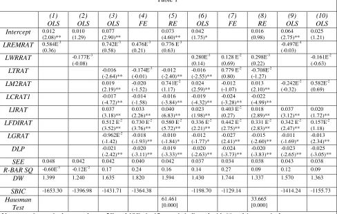
Before we estimate our modified production function we present estimates of the

conventional and standard specification of the growth equation used in many empirical

works. These estimates are given in Table 1. The dependent variable is the rate of growth

of per worker output (∆LYL). In columns (1) and (2) of Table 1 OLS estimates of with 2

definitions of remittances with pooled sample (OLS hereafter) are given. Since the sample

means are used in the estimation, pooled estimates can be treated as more satisfactory

proxies for the long run values of the variables. In column (1) growth rate is assumed to

depend only the ratio of remittances to GDP. One would expect that if remittances have

any significant long run growth effects the coefficient of remittances will be significant

and positive although it will be biased because other growth enhancing variables are

excluded and remittances may also depend on growth thus causing an endogenous

variable bias.6

Two definitions of remittances have been tried. The first is REMRAT which includes

remittances by all nonresidents and the second is WRRAT which includes remittances

only by nonresidents who are classified as residents in a foreign country and taxed there.

It is hard to say which of these two is better although Barajas et. al., assert that WRRAT is

better. Estimates of with these 2 measures of remittances are disappointing. While the

coefficients of REMRAT is positive it is insignificant. The coefficient of WRRAT is

6

Table 1 (1) OLS (2) OLS (3) OLS (4) FE (5) RE (6) OLS (7) FE (8) RE (9) OLS (10) OLS Intercept 0.012

(2.08)** 0.010 (1.29) 0.077 (2.90)** 0.073 (4.60)** 0.042 (1.75)* 0.016 (0.98) 0.064 (2.75)** 0.025 (1.21)

LREMRAT 0.584E-3

(0.36)

0.742E-3

(0.58)

0.476E-3

(0.21)

0.776 E-3

(0.63)

-0.497E-4

(-0.03)

LWRRAT -0.177E-3

(-0.08)

0.280E-3

(0.14)

0.128 E-2

(0.69)

0.298E-3

(0.22)

-0.161E-2

(-0.63)

LTRAT -0.016

(-2.64)** -0.174E-3 (-0.01) -0.012 (-2.40)** -0.016 (-2.55)**

0.779 E-2

(0.80)

-0.708E-2

(-1.27)

LM2RAT 0.019

(2.19)** -0.020 (-1.52) 0.741E-2 (1.17) 0.024 (2.59)** -0.012 (-1.07) 0.013 (2.10)** -0.242E-2 (-0.32) 0.582E-2 (0.69)

LCRAT1 -0.017

(-4.72)** -0.014 (-1.58) -0.016 (-3.84)** -0.019 (-4.32)** -0.024 (-3.28)** -0.022 (-4.99)**

LIRAT 0.037

(3.18)** 0.033 (2.26)** 0.040 (6.83)** 0.023 (1.98)**

0.403 E-2

(0.27) 0.018 (2.89)** 0.037 (3.12)** 0.020 (1.72)**

LFDIRAT 0.512 E-2

(3.52)**

0.730 E-2

(3.76)**

0.580 E-2

(5.72)**

0.336 E-2

(2.21)**

0.442 E-2

(2.75)**

0.331 E-2

(2.83)**

0.342 E-2

(2.47)**

0.157E-2

(1.18)

LGRAT -0.962E-2

(-1.42) -0.018 (-1.93)** -0.010 (-1.84)* -0.012 (-1.77)* -0.027 (2.41)** -0.015 (-2.60)** -0.011 (-1.69)* -0.013 (2.34)**

DLP -0.021 (-2.42)** -0.020 (-3.11)** -0.019 (-3.33)** -0.020 (-2.63)** -0.024 (-3.73)** -0.020 (-3.83)** -0.023 (-2.65)** -0.025 (-3.05)**

SEE 0.048 0.042 0.042 0.040 0.042 0.037 0.034 0.038 0.043 0.038

R-BAR SQ -0.60E-3 _-0.12E-2 _{0.17 0.24 0.16 0.14 0.27 0.09 0.12 0.09}

DW 1.399 1.240 1.635 1.820 1.594 1.430 1.744 1.337 1.570 1.363

SBIC -1653.30 -1396.98 -1431.71 -1364.38 -1198.70 -1129.14 -1414.24 -1155.73

Hausman Test 61.461 [0.000] 33.665 [0.000]

Notes: t-ratios are in the parentheses. 5% and 10% significance is indicated with ** and * respectively.

significant at the 10% level but it is negative. Addition of the lagged dependent variable

to these specifications did not yield better estimates. Similarly addition of squared

remittances, time trend and a multiplicative variable of remittances and M2RAT did not

yield a significant positive coefficient for remittances and these are not reported to

conserve space.7

We have added then some standard control variables to the above specifications.

These control variables, in their logs, are: trade openness (LTRAT), measured as the ratio

of exports plus imports to GDP, ratio of M2 definition of money to GDP (LM2RAT), ratio

of bank credit to private sector to GDP (LCRAT1), ratio of investment to GDP (LIRAT),

ratio of foreign direct investment to GDP (LFDIRAT), ratio of current government

expenditure to GDP (LGRAT) and the rate of inflation (∆LP).8 The specifications, with the expected signs for the coefficients, are as follows.

7

We followed here the alternative specifications tried by Barajas et. al.

8

0 1 2 3 4

5 6 7 8

0 1 2 3 4

2 1

(xx=7)

2 1

ti it it it it

it it it it

ti it it it it

LYL LREMRAT LTRAT LM RAT LCRAT

LIRAT LFDIRAT LGRAT LP

LYL LWRRAT LTRAT LM RAT LCRAT

α β β β β

β β β β

α β β β β

∆ = + + + +

+ + + + ∆

∆ = + + + +

5 6 7 8

1 6 7 8

(yy=8)

0 and and 0.

it it it it

LIRAT LFDIRAT LGRAT LP

β β β β

β β β β

+ + + + ∆

≥ ≤

These 2 equations are estimated with OLS and as fixed effects (different intercepts

but same slopes, FE hereafter) and random effects (RE hereafter) models.9 These 3 estimates for equation (7) are in columns (3), (4) and (5) and for equation (8) in columns

(6) to (8). For equation (7) the null in the Hausman test that the RE model is preferable

to the FE model is rejected. The test statistic, with the p-value in the square brackets, is

2

(6) 33.665 [0.00]

χ = and significant at the 5% level. However, the absolute value of SBI

of OLS estimate for this equation is higher at -1169.6 than the SBI for the FE model

which is -1129.1, thus favouring the OLS estimate in column (3). These results are also

valid for the estimates of (8) and its OLS estimate in column (6) is preferable to those in

columns (7) and (8).

In the preferred OLS estimate in column (3) out of the 8 slope coefficients 6 are

significant. It should be noted that the coefficient of remittances is insignificant although

its sign is positive. The signs of the coefficients trade openness and the credit ratio are

negative but significant at the 5% level and contrary to prior expectation. The signs of the

coefficients of the ratios of M2, investment, foreign direct investment to GDP and

inflation are as expected and significant. The sign of the ratio of government expenditure

has the correct negative sign but significant only at the 16% level. These observations

also hold for the OLS estimate of equation (8) in column (8) except that the ratio of

government expenditure to GDP now became significant at the 10% level. Although OLS

100 and if anyone finds the right set of control variables that would be a miracle. Therefore, our selection of these control variables should be treated with the usual caution.

9

estimates are preferred, the FE and RE estimates of these two equations are qualitatively

similar. OLS re-estimates of equations (7) and (8) after deleting the variables with the

wrong signs, viz., LTRAT and LCRAT1 are in columns (9) and (10). In neither equation

the coefficient of remittances is significant.10 Thus our estimates imply that the growth effects of remittance seem to be small and insignificant and support the findings in some

earlier works like Barajas et. al.

A weakness in the conventional specifications and estimates is that there is no

distinction between the short and long run effects of remittances or any other growth

enhancing variable. Since several empirical studies claim that they are analyzing the long

run growth effects of remittances and/or other growth improving variables, we shall use,

as discussed in Section 2, our extended specification in equations (3) and (5) based on

the Solow model. Besides the ratio of remittances we have included 7 other variables that

may have long run growth effects. These are shown in equations (7) and (8). Therefore,

the Z vector consists of 8 variables and an intercept to capture the growth effects of

trended but ignored variables. Our modified production function is:

( 1 )

0 (9)

i it

g g Z T

t t

y = A e +∑ kα

the vector Z_itconsists of the 8 variables from equation (7) or (6).

10

We have also tried estimates by instrumenting remittances with time trend and 2 and 3 period legged values of remittances. The correlation coefficient between remittances and the instruments was high at 0.88. Although the coefficients of REMRAT and WRRAT were positive in some estimates, they were

The specification in (9) cannot be easily estimated with the standard panel data

methods of OLS or FE or RE because of the nonlinearity of the variables. Generalized

Method of Moment (GMM) proposed by Arellano and Bond (1991) is the commonly

employed estimation procedure to estimate the parameters in a dynamic panel data model

with nonlinearities in the variables. In this method first differenced transformed series are

used to adjust for the unobserved individual specific heterogeneity in the series. But

Blundell and Bond (1998) found that this has poor finite sample properties in terms of

bias and precision, when the series are persistent and the instruments are weak predictors

of the endogenous changes. Arellano and Bover (1995) and Blundell and Bond (1998)

proposed a systems based approach to overcome these limitations in the dynamic panel

data models. This method uses extra moment conditions that rely on certain stationarity

conditions of the initial observation. The systems GMM estimator (SGMM) combines the

standard set of equations in first differences with suitably lagged levels as instruments,

with an additional set of equations in the levels with lagged first differences as

instruments; see for further details on the advantages of SGMM Arellano, Bond and

Temple (2002), Rao, Tamazian and Singh (2009) and Rao, Tamazian and Kumar (2009).

We shall use this estimation method to estimate our modified production function (8).

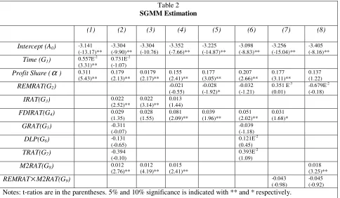
Our empirical results with SGMM are in Table 2. Due to the non-balanced nature of

our data we have ignored the first 5 years 1960 to 1964 and also the last 3 years 2005,

2006 and 2007. Therefore our sample covers the period 1965 to 2004. Furthermore, we

have encountered convergence problems due to high first order serial correlation in the

residuals of the levels equation. The estimated first order serial correlation is close to

unity. To achieve convergence the levels equations is estimated in a transformed form

where the first order serial correlation is fixed at 0.998.

We estimated first a simple version of equation (8) where TFP is assumed to be a

function of time only to get an understanding of the strength of TFP effects on growth

and also to check if this specification yields a plausible estimate for the share of profits

.

α The levels version of the estimated specification is:

where T is time. The estimates are in column (1) of Table 2. It can be seen that all the

parameters are significant at the 5% level. The estimate of profit share at 0.311 is highly

plausible and close to its stylized value of one third in the growth accounting exercises.

The coefficient of time implies that the long run growth rate of per worker income is low

in these countries at about 0.56%.

Table 2

SGMM Estimation

(1) (2) (3) (4) (5) (6) (7) (8)

Intercept (A0) -3.141

(-13.17)** -3.304 (-9.90)** -3.304 (-10.76) -3.352 (-7.66)** -3.225 (-14.87)** -3.098 (-8.83)** -3.256 (-15.04)** -3.405 (-8.16)**

Time (G1) 0.557E -2

(3.31)**

0.731E-2

(-1.07)

Profit Share (α) 0.311 (5.43)** 0.179 (2.13)** 0.0179 (2.17)** 0.155 (2.41)** 0.177 (3.05)** 0.207 (2.66)** 0.177 (3.11)** 0.137 (1.22)

REMRAT(G2) -0.021

(-0.55)

-0.028 (-1.92)*

-0.032 (-1.21)

0.351 E-3

(0.01)

-0.679E-2

(-0.18)

IRAT(G3) 0.022

(2.52)** 0.022 (3.14)**

0.013 (1.44)

FDIRAT(G4) 0.029

(1.35) 0.028 (1.55) 0.081 (2.09)** 0.039 (1.96)** 0.051 (2.02)** 0.031 (1.68)*

GRAT(G5) -0.311

(-0.07)

-0.039 (-1.18)

DLP(G6) -0.131

(-0.65)

0.121E-2

(0.45)

TRAT(G7) -0.394

(-0.10)

0.393E-2 (1.09)

M2RAT(G8) 0.012

(2.76)** 0.012 (4.19)** 0.015 (2.41)** 0.018 (3.25)**

REMRAT×M2RAT(G9) -0.043

(-0.98)

-0.045 (-0.92)

Notes: t-ratios are in the parentheses. 5% and 10% significance is indicated with ** and * respectively.

To understand on what factors TFP may depend it is necessary to estimate our

extended specification. We have estimated (8) with the 7 growth inducing variables in

the Z vector and the specification of this equation analogous to (9) is as follows.

1 2 3 4

6 7 8

1 6 7 8

5

ln ( 2 1

(10)

g 0 and g and g 0.

) T+ lnk

ti it it it

it it it

it it

y g g TRAT g M RAT g CRAT

g FDIRAT g GRAT g LP

g g IRAT π α = + + + + + + + ∆ ≥ ≤ + ×

In the first instance REMRAT is excluded from the specification for two reasons.

Firstly, variables like M2RAT, CRAT1 and IRAT are important channels through which

REMRAT is generally considered to have its growth effects. Therefore, adding REMRAT

may not produce good and reliable results because of multi-colinearity. Secondly, it is

affecting adequately TFP. If they do have significant growth effects, then it is likely that

1

g will be small or insignificant and remittances may indirectly improve growth through

these channels. We have excluded CRAT1 because its presence made its coefficient and

that of M2RAT insignificant. Estimates of (10) with the other 6 variables are in column

(2) of Table 2. Of these the coefficients only those of IRAT and M2RAT are significant at

the 5% level and they seem to explain adequately the trend in TFP because, as expected

above, the coefficient of trend g₁ is insignificant. However, the share of profits has

decreased to about 0.18 from its earlier estimate of 0.311 but this lower estimate plus 2 of

its standard deviations is not far below the stylized value of one third. Removal of trend

and 3 other insignificant variables with lower t-ratios viz., GRAT, DLP and TRAT has

improved the significance of the coefficient of FDIRAT and it is now significant at

slightly more than the 10% level. The reestimated equation is in column (3) of Table 2.

There are no significant changes in the estimates of the other parameters. These estimates

imply that the permanent positive growth effects IRAT, M2RAT and FDIRAT are small.

At the sample mean values of these variables of 0.21, 0.41 and 0.02, respectively, their

permanent growth effects are 0.44, 0.51 and 0.05 percentage points respectively. If IRAT,

M2RAT and FDIRAT can be increased by 50 percent, this will add about a 1.5 percentage

points to the long run growth rate of per worker output. Although this is a difficult target

it is not impossible to achieve. It is an attractive policy option because the average growth

rate of these countries is low at about one percent and this can be increased to 2.5 percent.

To examine if remittances has any growth effects the above equation is reestimated

by adding REMRAT and these are in column (4) of Table 2. It can be seen that the

coefficient of REMRAT has the wrong sign and is insignificant. When WRRAT is used in

place of REMRAT the results are similar and these are not reported to conserve space.

The insignificance of REMRAT may be because the growth effects of remittances

are indirect through its effects on variables like IRAT and M2RAT. Since these two are

already included in these estimates, REMRAT may not have any additional growth

effects. To test this we estimated this equation by removing both the channels viz., IRAT

and M2RAT and the results are in column (5) of Table 2.The coefficient of REMRAT is

negative and significant at slightly higher than the 5% level. The coefficient of FDIRAT

Addition of other non-channel variables GRAT, DLP and TRAT did not change the

results but the coefficients of these 3 variables are insignificant. These estimates are in

column (6) of Table 2. In this equation only the coefficients of FDIRAT and profit share

are significant besides the intercept. The coefficient of REMRAT is negative and

insignificant. When WRRAT is used in place of REMRAT it made no difference and these

are not shown to conserve space.

Recently Giuliano and Ruiz-Arranz (2009) have added a conditional multiplicative

term to show that remittances have positive growth effects and this effect is higher in

countries with less developed financial sector. This is plausible if remittances are a good

substitute for bank finance for funds to investment. In their SGMM estimate the

coefficient of REMRAT was positive (0.406) and the coefficient of the product of

REMRAT and the ratio of deposits to GDP was negative (-0.008) and both are significant

at the 5% level. To test if this result holds in our sample with an improved specification to

capture the long term growth effects, a multiplicative term REMRAT×M2RAT, which is

similar to the Giuliano and Ruiz-Arranz variable, has been added to the equation in

column (5). In this equation FDIRAT is the only control variable because the coefficients

of 3 additional non-channel variables, viz., GRAT, FDIRAT and DLP are found to be

insignificant; see estimates in column (6). Estimates with the multiplicative term are in

column (7) of Table 2. The coefficients of REMRAT and REMRAT×M2RAT have the

expected positive and negative signs but are highly insignificant. There is no other

significant change in the estimates of other parameters. When WRRAT is used in place of

REMRAT results were worse and the share of profits became insignificant. We have

added to this equation M2RAT as an additional variable although it is hard to justify

because it is a channel for REMRAT to affect growth and adding this or similar channels

is redundant and biases estimates. Nevertheless, since Giuliano and Ruiz-Arranz’s

specification includes a similar term and additional channels we estimated in column (8) a

specification with both REMRAT and M2RAT. Although the coefficient of M2RAT is

positive and significant the coefficients of REMRAT and the multiplicative term have

remained insignificant. Furthermore, the coefficient of REMRAT became negative and the

significance of other coefficients has worsened. In our view the standard specification

used by Giuliano and Ruiz-Arranz in which the unobservable long term growth rate is

proxied with 5 year average growth rate of GDP is unsatisfactory. Easterly et. al., (2004)

5 year average growth rate may be capturing some transient growth effects, whereas our

specification is more appropriate to estimate the effects on the long run steady state

growth rate. Therefore, it is difficult to accept that Giuliano and Ruiz-Arranz have

actually estimated the permanent long run growth effects of REMRAT in spite of their

elaborate but ad hoc specifications with a large number of multiplicative terms.

Nevertheless, their contribution is significant in many other respects because their data

refinements and use of SGMM and threshold effects techniques will encourage others to

follow their example, hopefully with improved specifications.

On the basis of these results it is hard to say that remittances have any long run

growth effects. However, as Giuliano and Ruiz-Arranz’s work reveals remittances may

have transient growth effects in the short run. Such effects are better suited for estimation

with country specific time series data and time series methods. These transient effects

may be significant and persist for a few years. If so, they will have significant permanent

level effects on per worker output. Furthermore, remittances may also have indirect and

permanent growth effects through its effects on IRAT and M2RAT etc However, these

growth effects are likely to be small because they will be the product of 2 fractions. For

example if the coefficient of REMRAT in the investment equation is 0.15 and significant

in a properly specified investment equation, since the coefficient of IRAT in our estimates

is 0.022, the indirect growth effect of remittances will be only 0.003. A 20% increase in

remittances will add an additional growth rate of only 0.07 percent. If these indirect

growth effects exist for REMRAT, they may be complex to untangle because as noted by

Barajas et. al., some are positive and some are negative. In our reduced form estimates the

coefficient of remittances when significant was negative; see column (5) of Table 2.

4. Conclusions

In this paper we have analyzed the direct growth effects of remittances and the

growth effects of the channels through which remittances may affect growth by treating

as conditioning variables. We have used conventional panel data estimation methods and

also the system GMM in which the limitations due to weak instruments and persistence in

the variables are minimized if not totally eliminated; see Buny and Windmeijer (2009) for

the weak instruments problem in SGMM. Our results showed that remittances, measured

However, we found 2 channels through which remittances may have indirect growth

effects. These are IRAT and M2RAT and both have direct growth effects. To estimate the

indirect growth effects of REMRAT through these channels, it is necessary to use proper

specifications for IRAT and M2RAT instead of arbitrarily regressing them on a single

variable such as REMRAT. This task is beyond the scope of this paper. We think that

such effects will be small in properly specified investment and money supply equations.

Therefore the ultimate growth effects of remittances through these channels will be also

small. Barajas et. al., offer a reason for this.11 According to them remittances, however small, may have both positive and negative effects on growth. The negative effects are

due to the Dutch Disease and deterioration of the quality of governance and neither of

them have been investigated in our paper. Therefore, these two effects may offset each

other if reduced form growth equations with remittances as the only explanatory variable

are estimated. While adding additional conditional variables it is appropriate to exclude

the channels through which remittance have indirect growth effects.

We agree with Easterly et. al., (2004), Rogers (2003) and Demirgüç-Kunt and Levine

(2008) on their criticisms of the specifications used in empirical growth models.

Therefore, We have suggested and estimated an extended production function, instead of

a growth equation, to derive the SSGR using the framework of the Solow growth model.

In many empirical works there is no awareness that the SSGR is an unobservable

variable—like the natural rate of unemployment. Both should be derived by estimating a

theoretically sound model by imposing the steady state conditions.

Although we found that remittances have no long run growth effects, they may have

short to medium term transitory growth effects. These growth effects do not raise the

permanent growth rates but they will have permanent level effects. We take the view that

cross country and panel data methods are less likely to be useful for estimating the

transitory growth effects compared to their estimates with country specific data and time

series methods. We hope that some investigators will pay attention to the significance

11

such level effects of remittances instead of concentrating solely on its long run growth

effects because these transitory effects persist for a few years and can permanently

Data Appendix: Data definitions and sources

Variables Definition Source

CRAT1 Domestic credit provided

by banking sector (% of GDP)

World Development Indicators (WDI) 2008

FDIRAT Foreign direct investment

to GDP ratio.

World Development Indicators (WDI) 2008

GRAT General government final

consumption expenditure to GDP ratio.

World Development Indicators (WDI) 2008

H Human capital; An average

of the Barro-Lee and Cohen-Soto data set and it incorporates a 7 percent rate of Return to each year of education.

Barro-Lee and Cohen-Soto data set.

IRAT Gross domestic fixed

investment to GDP ratio.

World Development Indicators (WDI) 2008

K Capital Stock; Derived

using perpetual inventory method

Kt = .95 * Kt-1 + It.

It is real gross domestic

fixed investment

International Financial Statistics, IMF

L Labour Force World Development

Indicators (WDI) 2008

M2RAT Money and quasi money

(M2) to GDP ratio.

World Development Indicators (WDI) 2008

DLP Inflation, (GDP deflator)

annual percentage

World Development Indicators (WDI) 2008

REMRAT Workers’ remittances and

compensation of

employees to GDP ratio. Workers' remittances and compensation of

employees comprise current transfers by

migrant workers and wages and salaries earned by nonresident workers. Workers’ remittances are classified as current private transfers from migrant workers who are residents of the host country to recipients in their country of origin. They include only transfers made by workers who have been

living in the host country for more than a year, irrespective of their immigration status. Compensation of

employees is the income of migrants who have lived in the host country for less than a year.

TRAT Sum of export plus import

of goods and services to GDP ratio.

World Development Indicators (WDI) 2008

WRRAT Workers’ remittances to

GDP ratio. Workers' remittances are current transfers by migrants who are employed or intend to remain employed for more than a year in another economy in which they are considered residents.

World Development Indicators (WDI) 2008

Y Real Gross Domestic

Product

References

Acosta, P., Lartey, E., and F. Mandelman (2007) Remittances and the Dutch Disease,

Federal Reserve Bank of Atlanta WP 2007-8.

Adams, R., and J. Page (2005) Do International Migration and Remittances Reduce

Poverty in Developing Countries?, World Development, 33(10): 1645-69.

Aggarwal, R., Demirguc-Kunt, A. and M. Peria (2006) Do Workers’ Remittances

Promote Financial Development?, World Bank Policy Research Working Paper 3957,

Washington, D.C.

Amuedo-Dorantes, C., and S. Pozo (2004) Workers’ Remittances and the Real Exchange

Rate: A Paradox of Gifts, World Development, Vol. 32(8): 1407-1417

Ang, J., (2008) A Survey of Recent Developments in the Literature of Finance and

Growth, Journal of Economic Surveys, vol. 22(3), 536-576,

Arellano M., and O. Bover (1995): Another Look at the Instrumental Variables

Estimation of Error-Component Models, Journal of Econometrics, 68, 29-51.

Arellano, M., and S. Bond (1991): Some Test of Specification for Panel Data: Monte

Carlo Evidence and an Application to Employment equations, Review of Economic

Studies 58, 277-297.

Barajas, A., Chami, R., Fullenkamp, C., Gapen, M., and P., Montiel (2009) Do Workers’

Remittances Promote Economic Growth?, International Monetary Fund Working Paper

No. WP/09/153

Blundell, R., and S. Bond (1998): Initial Conditions and Moment Restrictions in Dynamic

Burnside, C., and D. Dollar (2000) Aid, Policies, and Growth, American Economic

Review, 90 (4): pp. 847–868.

Buny, M., and F. Weindmeijer (2009) Problem of the System GMM Estimator in

Dynamic Panel Data Models, Econometrics Journal (Forthcoming) volume 12, pp.1-32

Chami, R., Barajas, A., Cosimano, T., Fullenkamp, C., Gapen, M.,and P. Montiel (2008)

Macroeconomic Consequences of Remittances, Occasional Paper No. 259, International

Monetary Fund

Dollar, D., and Kraay, A. (2004) Trade, growth and poverty, Economic Journal,

114(493), F22–F49.

Durlauf, S., Johnson, P., and J. Temple (2005) Growth econometrics. In Aghion, P., and

Durlauf, S. (Eds.), Handbook of Economic Growth, vol. 1, pp. 555–677. Chapter 8, pp.

555-677.

Demirgüç-Kunt, A., and R. Levine (2008) Finance and Economic Opportunity, World

Bank Policy Research Working Paper No. 4468

Easterly, W., Levine, R., and D. Roodman, (2004) New data, New doubts: A Comment

on Burnside and Dollar's “Aid, Policies, and Growth”, American Economic Review, 94

(3), 774–780.

Edwards, S., (1998): Openness, Productivity and Growth: What Do We Really Know?,

Economic Journal,108(447), 383-98.

Greiner, A., Semler, W. and G. Gong (2004) The Forces of Economic Growth: A Time

Series Perspective, Princeton, NJ: Princeton University Press.

Giuliano, P., and M. Ruiz-Arranz (2009) Remittances, Financial Development,

and Growth, Journal of Development Economics, 90, 144-152.

Gupta, S., Pattillo, C., and S. Wagh (2009) Effect of Remittances on Poverty and

Financial Development in Sub-Saharan Africa, World Development, Vol. 37(1), pp.

104-115

Hnatkovska, V., and N. Loayza (2003) Volatility and Growth, World Bank Working

Paper No. WPS3184.

Insights (2006) Sending money home: Can remittances reduce poverty?, Institute of

Development Studies, University of Sussex

International Monetary Fund (2005) Two Current Issues Facing Developing Countries, in

World Economic Outlook, April 2005: Globalization and External Imbalances, World

Economic and Financial Surveys (Washington).

Jones, C., (1995) R&D Based Models for Economic Growth, Journal of

Political Economy, 103: 759-784

Kroft, K., and H. Lloyd-Ellis (2002) Further Cross-Country Evidence on the Link

Between Growth, Volatility and Business Cycles, Queens University Working Paper.

Kohcerlakota, N., and Kei-Mu, Yi (1996) A Simple Time Series Test of Endogenous vs.

Exogenous Growth Models: An Application to the United States, Review of Economics

and Statistics, 78 (1), 126–134.

Lartey, E., Mandelman, F. and P. Acosta (2008) Remittances, Exchange Rate Regimes,

and the Dutch Disease: A Panel Data Analysis, Federal Reserve Bank of AtlantaWorking

Paper 2008-12

Lopez, H., Molina, L. and Bussolo, M. (2007) Remittances and Real Exchange Rate,

World Bank Policy Research Working Paper 4213, Washington: D.C.

Mankiw, N. G., D. Romer and D. N. Weil (1992) A Contribution to the Empirics of

Parente (2001) The Failure of Endogenous Growth, Knowledge, Technology and

Policy, 13: 49-58

Ramey, G., and V. A. Ramey (1995) Cross-Country Evidence on the Link Between

Volatility and Growth, American Economic Review, December 85(5), pp. 1138 – 1151

Ratha, D., (2003) “Workers’ Remittances: An Important and Stable Source of External

Development Finance,” in Global Development Finance 2003 (Washington: World

Bank).

Rogers, M., (2003) A Survey of Economic Growth, Economic Record 79 (244), 112–135.

Rao, B. B. (2006) Investment Ratio and Growth, ICFAI Journal of Applied Economics 3:

68-72.

Rao, B., and A. Cooray (2008) Growth literature and policies for the developing

countries, MPRA Paper 10951, University Library of Munich, Germany

Rao, B. B., Tamazian, A. and R. Singh (2009) What is the Long Run Growth Rate of the

Asian Tigers?, MPRA Paper 12668, University Library of Munich, Germany,

forthcoming, Applied Economics Letters.

Sato R (1963). Fiscal Policy in a Neo-Classical Growth Model: An Analysis of

Time Required for Equilibrium Adjustment, Review of Economic Studies 30: 16-23

Siddiqui, R., and A. R. Kemal, (2006): Remittances, Trade Liberalisation, and Poverty in

Pakistan: The Role of Excluded Variables in Poverty Change Analysis, The Pakistan

Development Review, vol. 45(3), pages 383-415.

Solow, R. (1956): A Contribution to the theory of economic growth, Quarterly Journal of

Economics, 70(1), 65-94.

Solow, R. (2000). Toward a Macroeconomics of the Medium Run, Journal of

World Bank (2006) The Development Impact of Workers’ Remittances in Latin America,