Evaluating alternative methods for testing asset pricing models with historical data

Munich Personal RePEc Archive

Evaluating alternative methods for

testing asset pricing models with

historical data

Rubio, Gonzalo and Lozano, Martin

Universidad CEU Cardenal Herrera, Universidad del País Vasco

8 September 2009

Online at

https://mpra.ub.uni-muenchen.de/23613/

Evaluating Alternative Methods for Testing

Asset Pricing Models with Historical Data

Martín Lozano Universidad del País Vasco

[email protected]

Gonzalo Rubio

Universidad CEU Cardenal Herrera

[email protected]

September 8, 2009

Key Words: Beta Pricing Models, Stochastic Discount Factor, Pricing Errors, Evaluation of Factor Models.

JEL classification: C51, C52, G12 _________________________________

The authors thank participants in the XV Foro de Finanzas at Universidad Islas Baleares, and especially Belén Nieto, Rosa Rodríguez and Miguel A. Martínez for helpful comments and suggestions, and seminars participants at Universidad del País Vasco. We are especially indebted to an anonymous referee for his thoughtful suggestions which greatly improved the paper. Martín Lozano acknowledges financial support from Consolidate Research Team 9/UPV-00038.321-15094/2001 and Gonzalo Rubio acknowledges financial support from Generalitat Valenciana grant PROMETEO/2008/106, and Ministerio de Ciencia e Innovación grant MEC ECO2008-03058/ECON.

Abstract

1. Introduction

Asset pricing literature has been debating between reduced-form portfolio-based models or factor models, where marginal utility of consumption is directly measured by the returns on a few number of large portfolios, and macroeconomic models, where the focus is on understanding the marginal utility that drives asset prices.1 In this paper, we concentrate on the former. In particular, we analyze models linking excess returns to the returns of orthogonal factor-mimicking portfolios (or simply factors).

Recent empirical evidence tends to find that not only the market but other aggregate risk factors seem to be important in describing the cross-sectional variation of average returns. Fama and French (1993, FF hereafter) introduce a three-factor model by adding a market capitalization (size) and a book-to-market (value) factor to the CAPM excess market factor return. Furthermore, Carhart (1997) proposes a four-factor model by appending the three FF factors with a momentum factor after the study by Jegadeesh and Titman (1993) on returns to momentum strategies.

These risk-return models have been extensively tested in the finance literature by the regression based “traditional method” or Beta method, in which a cross-sectional regression model is proposed for average stock returns, and the theoretical implications are tested as hypothesis on the parameters of the regression model.2 However, it is well known that linear asset pricing models such as CAPM or FF, and many others, including nonlinear specifications, can be unified in a stochastic discount factor (SDF) framework. This involves estimating the asset pricing model using its SDF representation and, in most cases, the generalized method of moments (GMM).

The comparison of the two methods (Beta and SDF) is not an easy matter even for linear models, since the parameters of interest are different under the two setups. The Beta method is formulated to analyze the factor risk premia, and these are the primary parameter of interest. In contrast, the SDF representation is formulated to analyze the parameters that enter into the imposed SDF. The first formal comparison between the two methods is performed by Kan and Zhou (1999). They argue that the SDF is inferior

1

See Cochrane (2008) for a detailed and provocative discussion on these fundamental issues.

2

to the traditional maximum likelihood approach, even in a simple test of the CAPM, as long as returns are identical and independent normally distributed random variables. Jagannathan and Wang (2002, JW hereafter) show, in a very influential paper, that Kan and Zhou´s conclusions are incorrect. These authors fail to explicitly incorporate the transformation between the risk premium parameters in the two methods, and they ignore the information about the mean and the variance of the factor while estimating the risk premium. Once this is done, JW (2002) analytically show that the SDF method is as asymptotically efficient as the Beta method. At the same time, their empirical exercise, based on a set of simulations under the CAPM framework, also find similar results for both methods. They assume that the returns of 10 size-sorted portfolios and the market factor are drawn from a multivariate normal distribution, considering four different time horizons. Moreover, they also demonstrate that the SDF method has the same power as the Beta method.3 Cochrane (2005) also show that using 10 size-sorted portfolios, a given sample period and the simple CAPM case, the two methods produce basically the same standard errors, t-statistics, and 2statistics that the pricing errors are jointly zero.

In this paper, we follow the correct JW (2002) framework for comparing the estimates and specification tests of the classical Beta and SDF methods, using historical data instead of simulations. Furthermore, and contrary to Cochrane (2005), we test not only the single factor model but also the FF three-factor model, and an alternative specification based on the excess market return, and the value and momentum factors (the RUH model hereafter). In fact, the main contribution of this paper is the performance of a comprehensive extension of the analysis reported by Cochrane (2005). From our point of view this covers an important gap in the empirical asset pricing literature. A relevant added value is the high number of sample and estimation technique combinations we employ in our research. We estimate three models, thirteen test portfolios, six time periods and eight econometric techniques. This turns out to be an appropriate approach to better understand the differences between the Beta and SDF/GMM methods. On the basis of the previous papers by JW (2002) and Cochrane (2005), it is generally accepted that the differences between the Beta and SDF/GMM methods are practically irrelevant in terms of specification tests and properties of

3

estimators. However, we show that this is not the case, once we generalize the evidence to multifactor models. For example, when estimating risk premia, the Beta method has better properties in multifactor models across test portfolios and sample periods than the SDF/GMM method, while the main consensus is that there no differences between both methods. Moreover, our results are not driven by a simulation calibrated from a single factor structure, as in JW (2002); they are obtained from actual realizations of historical data. This allows us testing the methodologies under more complex set-ups other than varying according to a known distribution. The closest paper is probably due to Shanken and Zhou (2007). However, once again, although the objective of the paper is similar, they report empirical results based only on simulations rather than on real data sets.

It is also the case that, in order to address the tight factor structure problem advocated by Lewellen, Nagel and Shanken (2009, LNS hereafter), it becomes very important to extend previous papers with similar objectives by adding a large number of test assets and time periods. LNS (2009) provide an interesting empirical exercise showing how asset pricing tests are often highly misleading. They demonstrate that if the set of test assets has returns with a strong factor structure, like size or book-to-market-sorted portfolios, almost any proposed factor weakly correlated with the FF factors is likely to produce betas that line up with average returns generating a high cross-sectional R2.

Our paper use six families of N test portfolios: 5 and 10 formed on ME (size); 5 and 10 formed on BE/ME (value); 6, 25 and 100 formed by the intersections of ME and BE/ME (FF portfolios); 6 and 25 formed on ME and MOM (size and momentum); 5, 17 and 30 industry portfolios, and an extended test assets case in which we simultaneously combine the 25 FF portfolios and 17 industry portfolios. In this way, we can be confident that our results are not driven by the factor structure argument of LNS (2009). We also conduct our analysis using 6 time horizons T of US tests portfolios: 60, 120, 240, 360, 480 (all of them to cover the post-1963 data) and 948 monthly observations (the longest time-series used in this paper which goes from January 1927 to December 2005).

Hansen and Jagannathan (1997, HJ hereafter); first and second-stage returns on covariances, following Cochrane (2005); and the continuous updating estimate following Hansen, Heaton and Yaron (1996, HHY hereafter). We are therefore interested on evaluating how (and if) the Jagannathan and Wang (2002) and Cochrane (2005) results change in this richer framework.

Our results provide new evidence about finite-sample setups in which SDF/GMM formulation lead to almost the same results as the Beta method and also others in which there are significant discrepancies. These differences emerge even in linear models. Therefore, it may not be necessary to have a hard set up such as highly nonlinearity in order to anticipate differences between the two methods. In particular, our evidence reveals that SDF/GMM first-stage estimators lead to lower pricing errors than OLS, while SDF/GMM second-stage estimators display higher pricing errors than the classical Beta GLS method. Moreover, the Beta method (OLS and GLS) seem to dominate the SDF/GMM (first and second-stage) procedure in terms of estimators’ properties. This implies that the Beta method tends to find risk premia estimates closer to the observed (ex-post) risk premia. In this sense we also follow the LNS (2009) recommendation about taking seriously the economic implications of the risk premia estimators. These results are consistent across benchmark portfolios and sample periods.

This paper is organized as follows. Section 2 briefly reviews the econometrics of estimating and evaluating asset pricing models. A full description of the data employed in the paper is presented in Section 3. Section 4 discusses the empirical results and a detailed analysis of different comparisons, while Section 5 concludes.

2. A Brief Description of the Beta and SDF/GMM Methods

of pricing errors and V is some weighting matrix.4 We now briefly describe the beta and the SDF procedures.

2.1 The Beta Method

We want to fit the following simple regression model

E R

 

e_j   _j  _j (1)

where Re_j is the excess return over the risk-free rate for any stock j, _j is a K-vector of sensitivities of stock j with respect to a set of aggregate risk factors,  is the vector of risk premia, _j is the pricing error, and E is the expectation operator. The idea is of course to learn why average returns vary across assets.

In this paper, this is done by running an OLS, WLS and GLS cross-sectional regressions of average returns on the betas. Since betas in (1) are estimated in a time-series regression, we correct asymptotic standard errors by applying the Shanken (1992) multiplicative correction



1  ˆˆ_f1ˆ



, where ˆ_f is the variance-covariance matrix of the factors. We finally test whether all pricing errors are jointly zero with the asymptotic OLS, WLS and GLS 2 test of pricing errors.

2.2 The SDF Method

It is well known that the first order pricing equation from the intertemporal optimization of the representative agent can be written as

p_t E m_t



_{t 1 t 1} x_



(2) where p_t is the price of any stock, m_{t 1} is the SDF which is the intertemporal marginal rate of substitution of consumption, x_{t 1} is the future payoff of the stock and is the conditional expectation operator. An asset pricing model identifies a particular SDF (a proxy for the marginal rate of substitution of aggregate consumption) that is a function of observable variables and the model parameters. The SDF method involves estimating the asset pricing model using its SDF representation and the GMM procedure.

t

E

4

The development of the GMM by Hansen (1982) has had a major impact on empirical research in finance because it allows for conditional heteroskedasticity, serial correlation and non-normal distributions. In this section, we review the estimation and testing of linear discount factor models expressed as,5

p E mx or 1

 

E mR

 

m b f

 



 (3)

This pricing expressions lead naturally to the GMM when testing asset pricing models, where the pricing errors are precisely the moments used in the estimation.

2.2.1 First and Second-stage GMM Estimators

The idea is to choose b to make the pricing errors g_T

 

b as small as possible, by minimizing the quadratic form,

(4)

  T

 

T

 

b

min g_ b Wg b _

When imposing W = I, GMM treats all test assets symmetrically, and we just minimize the sum of squared pricing errors. The result of making such simplification is what we call first-stage estimators. This estimator is consistent and asymptotically normal.

The second-stage estimate makes a formal statistical choice of the weighting matrix W. Since returns are correlated, the usual procedure chooses the variance-covariance matrix of E_T



m( b )R 1 



E_T



u( b )



g_T

 

b , so that the matrix pays more attention to linear combinations of moments for which the available data is more informative. Hansen (1982) shows formally that the choice W S1, where S 



__E u u



_{t t}_



is the optimal weighting matrix in the sense of having the lowest asymptotic variance.

2.2.2 Hansen and Jagannathan (1997): GMM Estimators _A

Another example of prespecified economically interesting weighting matrix is the second moment matrix of returns suggested by HJ (1997). In this subsection, we will refer to S as the second moment matrix of returns. They also introduce the Hansen-Jagannathan distance, which measure specification errors of SDF models by least

5

squares distances between an SDF model and the set of admissible SDFs that can correctly price a set of test assets.

Cochrane (2005) points out that when writing the model as m a b f , it is not possible to separately identify a and b, so we choose first the easiest normalization in which a = 1. Then, g ( b )_T  E_T

 

mRe  E_T

   

Re E R fe  b

 

. We employ the usual

notation, g b E R f

 

e b

T

d   

   , to get the second moment matrix of returns and

factors. The first order condition to minimize (4) is d W E _{ T}

 

Re db_0. The first

stage imposes W I, while the second stage uses W S1. Since the parameter b

enters linearly in the minimization, we can find their estimates analytically:

 

 







1 e 1 T 1 1 1 2 T ˆ

First Stage: b d d d E R

ˆ ˆ

Second Stage: b d S d d S E R

        

 e



(5)

Hence, the GMM_A estimate is a cross-sectional regression of mean excess return on second moment matrix with factors. The standard errors of and and the covariance matrix of the pricing errors

1

ˆb ˆb₂

 

T ˆ

g b are calculated following Hansen (1982).

The model test is a quadratic form in the vector of pricing errors g_T

 

b . Note that there are two ways to get a small value of the test statistic, usually denoted by . First and desirable, we can generate small pricing errors with a high degree of precision or, and this is not desirable, we can generate large pricing errors with even higher standard errors of those errors. Thus, in this paper we would care not only on specifications test results but also on the pricing errors themselves. Thus, in this paper we would care not only on specifications test results but also on the pricing errors in order to avoid this trap.

T

2.2.3 Cochrane (2005): GMM_B Estimators

Alternatively, we can run a cross-sectional regression of mean excess returns on covariances by choosing a normalization a 1 b E f

 

rather than a = 1. Then, the model is m 1 b_f E f

 

_ with mean E m

 

1. The pricing errors are,

g_T

 

b E_T

     

mRe E_T Re E_T R fe b (6)

where f  f E f

 

. We have d gT

 

b E

 

e b



R f

 



  , which now denotes the

covariance matrix of returns and factors. We must bear in mind that the mean of the factor E f

 

is estimated in (as well as b), and the distribution theory should recognize sampling variation induced by this fact as we usually do in the cross-sectional regressions. Second-stage estimators comes from the minimization of the following expression, B GMM (7)  







1 T T

b,E( f )

ˆ

min _g b,E( f ) S  g b,E( f ) _







which can be solved using a numeric method.6

2.2.4 Hansen, Heaton and Yaron (1996): GMM_CU (Continuous Updating) Estimators

Another possibility is estimating the spectral density matrix or, in other words, use the optimal weighting matrix instead of taking the prespecified weighting matrix on the second-stage estimators, as we advocate in GMM_A and . The iterated

estimator using the optimal weighting matrix may present two related problems. First, if the variance-covariance matrix for the iterated estimator is poorly measured, then the estimator will put too much weight on moments that spuriously appear to be measured precisely. Moreover, the iterated estimator may place too much weight on test assets that are economically uninteresting, in the sense of being extreme short and long positions in some of the stocks.

B GMM GMM CU GMM CU

Furthermore, the fact that the S matrix changes with the model, may improve the statistic because it blows up the estimate of S, rather than by lowering the pricing T

J

6

errors. As Cochrane (2005) emphasizes we should not compare formally tests across models. This is one of the reasons why it is recommended to use a common weighting matrix for comparing models like those discussed above. There are several alternatives to the second-stage procedure. We use the continuous updating estimator which states that it is not true that S must be held fixed as one searches for b. Instead, one can use a new for each value of b, and estimate b by

T

J

 

S b

 



gT

     

b S b gT b



b

1

ˆ '

min  (8) The estimates produced by this simultaneous search will not be numerically the same in a finite sample as the two-step or iterated estimates.

To wrap up, we have three econometric specifications in the beta method: OLS, GLS and WLS. And five in the SDF/GMM method: First and second stages of GMM_A,

, and the continuous updating . When estimating, we collect the central parameter (lambda for beta method and b for SDF method), standard errors and bias from the factor mean. On the other hand, when testing, we collect the pricing error and the p-value of the model specification test.

B

GMM GMM_CU

3. The Data

Three single (size, value, and industry), two double-sorted (value and size-momentum), and one combined (size-value plus industry) test portfolios are taken from the data library of Kenneth French because of familiarity and availability to the general readership.7 In sum, we take six types of N test portfolios: 5 and 10 formed on ME; 5 and 10 formed on BE/ME; 6, 25 and 100 formed by the intersections of ME and BE/ME (FF portfolios); 6 and 25 formed on ME and MOM; and 5, 17 and 30 industry portfolios. LNS (2009) suggest that one could expand the set of test portfolios to price all of them at the same time. In this paper, besides the previous five types of test assets, we use an extended set formed by 25 Fama-French portfolios plus 17 industry portfolios, resulting in a total of 42 test portfolios. Note that we take at least two different values of N within each test assets in order to provide the robustness checks.

7

We conduct our analysis using six values for the time length monthly observations T: 60 (January 2001-December 2005), 240 (January 1986-December 2005); 360 (January 1976-December 2005); 480 (January 1966-December 2005) and 948 (January 1927-December 2005). The choice for a monthly interval reflects the trade-off between the sampling error of a sufficiently large sample, and a realistic evaluation horizon. Increasing the return interval (e.g. yearly) would lead to a small data set, while decreasing it (e.g. daily) to an unrealistically short evaluation horizon. Further, the use of high-frequency data introduces well known microstructure problems which may distort the empirical results. Therefore, we adhere to the common approach of using monthly returns.

Taking into account the three models, thirteen test portfolios, six time periods and eight econometric specifications, we end up with 1636 and 2730 observations of lambda and

b estimators with their corresponding standard errors and bias from the factor mean. On the other hand, we have 702 beta and 1170 SDF observations of pricing errors with their corresponding p-values of the model specification test.8 This amount of results is a considerable expansion to similar previous works like Cochrane (2005) or Shanken and Zhou (2007), and thus we are clearly able to broaden the comparisons between the two methods. Our datasets include not only low but also high dispersion of tests assets returns, this imply that methods and models will be forced to price tests assets with high variance and low factor structure.

4. The Empirical Results

In this section, we first compare the pricing errors and model specifications of the Beta method with respect to the SDF/GMM method across models, test assets and time periods. Then, we perform the analysis regarding the properties of estimators. As in JW (2002) and Cochrane (2005), our results from testing and estimating the CAPM in the simple and classic set up illustrate that the differences between both methods are practically irrelevant.9 However, the key point is that we show how the differences become significant in a more complex setup.

8

Note that the number of outcomes from the beta method is always less than from the SDF procedure. This is because we have three specifications for beta, and five for the SDF. However, most of the comparisons conducted are based on similar numbers of observations.

9

4.1 A Comparison of Pricing Errors and Specification Tests.

In this subsection, we are concerned with two key issues. The first one regarding which method leads to lower pricing errors, while the second one analyzes how well that method does when testing the three models.

4.1.1 Which Method Leads to Lower Pricing Errors?

Let us begin analyzing which method leads to lower pricing errors by confronting first OLS and first-stage GMM_A SDFand, secondly, by making comparisons between GLS and the second-stage GMM_A SDF. We perform the analysis for CAPM, FF and RUH models and the test portfolios described on section 3; that is 360 pricing error observations for each method.

Table 1 summarize the results of comparing Beta versus GMM/SDF pricing errors, using four time periods from T = 240 to T = 948. Our results suggest that first-stage

A

GMM SDF dominates OLS, while GLS dominates second-stage GMM_A SDF at minimizing pricing errors, and this result is consistent across test portfolios and sample periods.10

The OLS and first-stage GMM estimators are intended to minimize the root mean square errors since there is no weighting matrix, but first-stage estimators do it better than OLS. The results contained in the second column of Table 1 tells us a different story; in this case Beta method does it better in achieving lower pricing errors than second-stage GMM estimators, even though these methods do not have the pure objective of minimizing the sum of square errors, as first-stage and OLS do. Interestingly, both results are obtained independently of the test assets employed. As an example, when using the extended set of 25 FF portfolios and 17 industry portfolios, the Beta/OLS method generates higher pricing errors than first-stage GMM_A SDF in all cases. On the other hand, only in 11 percent of the cases, the Beta/GLS method generates higher errors relative to second-stage GMM_A SDF.

10

4.1.2 Testing the Alternative Pricing Model Specifications

First-stage GMM_A SDF does a good job at minimizing squared pricing errors; hence we can now look at the test statistics with more confidence. A new question that arises is how different are the specification test results from first-stage GMM_A SDF when applied to three models, four time periods, and six families of test portfolios. In order to summarize the results, let us focus on the p-values and group them in quartiles by test portfolios and by models.

Our test results are summarized in Table 2. Each panel represents a particular asset pricing model: CAPM (upper), FF (middle) and RUH (lower). Columns from left to right in each panel are families of N tests portfolios formed by ME, BE/ME, ME & BE/ME, Industry, and the extended set of ME & BE/ME (or FF portfolios) plus Industry respectively. It should be recalled that each column is formed by at least two different values of N and four time-lengths. Rows are the probability intervals of not rejecting the null. Therefore, a column with larger proportion of the last interval 76-100 implies that the null will not be rejected in most cases for that model and test portfolio.

Table 2 shows the CAPM is rejected for all test portfolios more often than any other competing model. In particular, for the ME & BE/ME, ME & MOM, and the extended test assets, the rejection of the CAPM is absolute in the sense that all their tests have (1-p-values) between 0 and 25 percent. Our results show that when testing the CAPM with size-sorted portfolios, as in Cochrane (2005), only in 17 percent of the cases we report high probability of not rejecting the null.

able to price the ME & BE/ME, ME & MOM portfolios, and the expanded set of assets. Although the pricing errors are in fact lower, they are not enough for getting at least a portion of any other interval. Only the RUH specification is capable of successfully pricing 25 percent of the cases for the FF portfolios, and also reduces to 50 percent the cases in which the model can not price these portfolios at all.

Generally speaking, this evidence suggests that multifactor models help rather than hurt for all these test portfolios' valuations. The evidence seems to be slightly better for the RUH model relative to the FF model. The RUH model performance is particular remarkable since there is no track of this specification in previous literature. The probability of not rejecting the null is higher for every test portfolio and model tested under the RUH specification. However, it fails to price the set of extended assets.

Table 2 also suggest that the specification testing results depend on the test portfolios employed. It seems that portfolios' characteristics are driving the rejection of the null hypothesis. In particular, the dispersion of average returns across portfolios seems to be positively correlated with the pricing success of any given model. Returns on portfolios formed by ME has a cross-sectional standard deviation of 12 percent, 16 percent for BE/ME and Industry portfolios, 23 percent for the extended set of assets, 27 percent for ME & BE/ME, and 45 percent for ME & MOM. The double-sorted portfolios (e.g. FF, size-momentum, and the combined set) seem to be harder to price because they have significant higher dispersion than single-sorted portfolios. Note, for example, that when testing size and momentum sorted portfolios (ME & MOM), or the extended set, we cannot reject the null in any case. Their associated pricing errors are all statistically different from zero. They are, together with the FF portfolios, the test assets with higher cross-sectional dispersion.

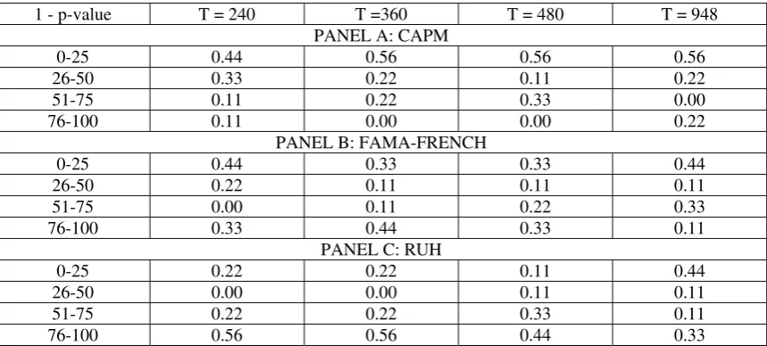
One may always think that the results reported in Table 2 are being drive by some particular characteristics of the historical data on a given time-period. Thus, we perform a robustness check by changing the perspective view over the same results. In Table 3, we now control for the sample period T r

as

ather than controlling for the test portfolios N

we did on Table 2. Then, the columns in Table 3 now represent time periods (instead of portfolios), and the rest is exactly the same as in Table 2.

This alternative representation of Table 2 allows us to analyze whether the evidence in favor of multifactor models reported before is independent of the time length. In this regard, it should be pointed out that some studies suggest that the choice of the sample period and size segment are important for judging the empirical validity of the CAPM.11 Our evidence suggest that the choice of the sample period is not relevant for evaluating the empirical validity of the CAPM and multifactor models, at least in tests of over identifying restrictions. It is true, however, that pricing errors diminish for longer time horizons. In this sense, our results are also consistent with those on Shanken and Zhou (2007).

4.2 A Comparison of Estimators’ properties.

We now turn from tests on pricing errors to evaluate the estimators' properties. Remember we are dealing with historical datasets. We understand that an estimator has desirable properties if it satisfies the following three conditions (1) it has low standard error, (2) it is statistically different from zero, and (3) it has low bias (measured as the percentage error) relative to the observable factor. In this subsection we follow the

correct framework for comparing estimates presented on JW (2002).

We are now concerned with the following two questions: Which method leads to better estimators' properties within methods (OLS versus GLS, and first versus second-stage)? Which method leads to better estimators' properties intra methods (OLS versus first-stage, and GLS versus second-stage)? We will answer these questions by aggregating by models, test portfolios and sample periods. Then, we are actually comparing 2184 estimators with their corresponding standard errors, t-statistics and percentage bias. Our

11

results suggest that, in general, the Beta method leads to better properties than the SDF/GMM method.

Due to the large number of lambda and b estimates, it is useful to classify their properties into three categories, in a similar way as we did before. For this purpose, we define the category A in Tables 4, 5 and 6 for those estimators who are less than 50 percent biased from the observable risk factor and are statistically different from zero. The category B corresponds to those estimators with biases between 51 percent and 100 percent whether or not they are statistically different from zero. Finally, the category C is for estimates with 101 percent to 1000 percent biases whether or not they are statistically different from zero. Few observations with a bias even higher than 1000 percent are dropped out from the analysis; it is worthwhile to mention that 95 percent of these dropped values correspond to SDF estimators. Naturally, the category A represents the best properties. By restricting to be statistically different to zero we guarantee that the standard error is relatively small, and the bias condition assures that the estimate is reasonable as LNS (2009) emphasize. In the category B, we are not interested on the size of the standard error; the only condition is the bias interval. Thus, the unreasonable estimates will fall into this category. The category C represents obviously the worst properties because their bias is extremely high; these estimators become not only unreasonable but also unreliable.

Table 4 shows that GLS leads to better properties than OLS, except for the industry portfolios in which category A goes from 48 percent in OLS to 41 percent in GLS. The rest of portfolios increase the category A between 4 to 10 percentage points. Thus, in general, GLS is actually doing its job at providing better properties by giving up some pricing errors. Furthermore, the category C is actually smaller for the GLS, strengthening the fact that GLS has better properties than OLS. This is true for all portfolios except again for the industry classification in which the category C goes from 27 percent in OLS to 32 percent in GLS. The rest show a decrease from 3 to 26 percentage points.12

12

On the other hand, the results regarding the second-stage relative to the first-stage estimators are less clear in achieving better properties. The second-stage estimators obtain better properties, except for the double-sorted portfolios in which the category A decreases from 27 percent (FF), 40 percent (size-momentum), and 29 percent (extended assets) in first-stage to 18, 17, and 8 percent respectively in second-stage. The rest have a modest improvement between 1 and 6 percentage points. The category C in second-stage is lower than in first-second-stage, except again for the double sorted portfolios which goes from 50 percent (FF), 32 percent (size-momentum), and 50 percent (extended assets) to 71, 59, and 80 percent in second-stage. The rest of them have a tiny improvement of 1 percentage point each. Note that the Beta method can achieve better estimators’ properties even in portfolios with high dispersion, while the SDF method cannot. This is consistent with the idea that GMM has difficulties in small samples. In our case this difficulty is associated with the higher dispersion in the portfolios’ expected returns. In other words, GMM seems to have difficulties in pricing assets when changing from single-sorted to double-sorted portfolios (including the set of extended test assets).

Regarding the second question, the Beta method dominates SDF in terms of estimators’ properties. The category A consistently becomes larger from first-stage to OLS and from second-stage to GLS. In particular, the increases go from 11 (size-momentum portfolios) to 45 (FF portfolios) percentage points. On the other hand, there is also a substantial decrease of the category C between 10 (value portfolios) to 68 (extended test assets) percentage points; in this case the only exception is the industry portfolios which slightly increases from 31 percent (second-stage) to 32 percent (GLS).

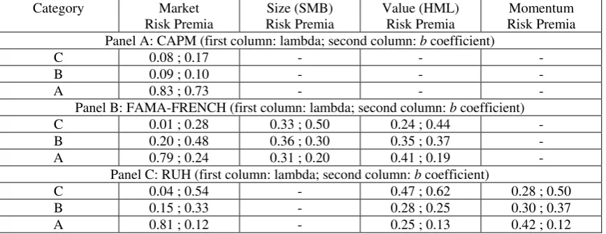
Our next task is therefore to compare the estimators' properties across models. Given that the Beta method dominates SDF, then, the next question is whether this evidence is consistent for each model and for all methods. For this purpose, we use an even broader set of estimators than before: we now calculate three kinds of estimators in a beta formulation: OLS, GLS and WLS; and five estimators in a SDF formulation: returns on second moments of HJ (1997); returns on covariances of Cochrane (2005); and the continuous updating estimate of HHY (1996). These estimations were obtained by taking our full sample on T and N. We finally end up with about 1636 lambda and 2730

b estimators.

The evidence is summarized in Table 5. Each panel represents the alternative factor models, while columns are lambda and b estimates’ properties. In each column we report the frequency of each category by factor (market, size, value and momentum). We drop some estimators with more than 1,000 percent bias from the factor mean. As before, it is worthwhile to point out that 95 percent of the 151 total dropped values correspond to the SDF. This already suggests which method is more likely to deliver an estimator with worst properties.

Let us focus on the first panel (CAPM) of Table 5. As in Jagannathan and Wang (2002) and Cochrane (2005), we find that the lambda and b associated with the market factor have almost identical properties in both methods, even in a more complex setup than the simple CAPM with 10 size-sorted portfolios. In particular, we find that the probability of having good properties is 83 and 75 percent for the Beta and SDF respectively. This result is remarkable because it is actually what JW (2002) show in their empirical results with simulated data, and we find very similar results using historical datasets.

In any case, why does the lambda and b estimates associated with the market factor have so similar properties in the CAPM and so different in multifactor models? One plausible answer is that b gives a multiple regression coefficient of m on the factor given the other factors; while lambda gives the single regression coefficient. In the CAPM model of course, there is no difference between single or multiple regression coefficient since there is only one factor. So, lambda and b behave in a very similar way as long as both report single regression coefficients, but things change when adding more factors.

The size factor from FF model and the momentum factor from RUH model are priced, and help pricing assets given the other factors, in a similar magnitude. That is, even though we find that Beta method lead to better estimators' properties than SDF, the difference is not as large as when comparing the market factor in the FF and RUH models. Finally, the results regarding the lambda and b associated with the value factor show similar results. The Beta method does achieve better properties than the SDF procedure. In the FF model, the category A is twice for lambda (41 percent versus 19 percent), and it is three times larger in the RUH specification (42 percent versus 12 percent).

As Amsler and Schmidt (1985) and Shanken and Zhou (2007), we find that when T is small (say 60 or 120), these estimators can be very volatile across different test portfolios. Thus, in Table 6 we exclude time lengths equal to 60, 120 and 240. When taking away the three smaller sample periods, we are actually dropping off the estimators with higher bias and standard errors, and then our conclusions about Table 5 strengthen. The properties regarding the multifactor models get better when dropping out the smallest time-periods. The category A is now consistently larger and the category C smaller than in Table 5.

5. Conclusions

known that GMM has difficulties in finite samples, when dealing with extreme nonlinearities; nonetheless we find that their difficulties can arise even in linear models.

We find that HJ (1997) first-stage GMM achieve lower pricing errors than OLS Beta method for all test portfolios and time-lengths. On the other hand, their specifications tests show evidence in favor of multifactor models such as RUH because the likeliness of not rejecting the null is greater than in FF and CAPM models. We also find that double-sorted portfolios are hardest to price compared with single-sorted portfolios, and this difference is correlated with the higher dispersion on the test portfolios’ average returns.

Theory indicates that GLS should lead to better estimators’ properties than OLS, and this should also apply to second and first-stage GMM estimators. Our results suggest that the beta method actually do better than the SDF method. Moreover, when pricing double-sorted portfolios, the properties on second-stage are actually worse than in first-stage.

We are capable to reproduce JW (2002) results for the CAPM even in a finite-sample framework, which reinforce the strength of the fact that there is no difference between Beta and SDF methods when comparing lambda and b properties under the simple CAPM. Our main contribution relies on extending the comparison for the FF and the RUH specifications. Our results imply that differences between the performance of the methods arises in more complex setups such as the ones suggested by LNS (2009). In particular lambda from the beta method has better properties in multifactor models such as FF and RUH than b from the SDF method across tests portfolios and sample periods.

References

Ang, A., and J. Chen (2007). "CAPM Over the Long-Run: 1926-2001", Journal of Empirical Finance 14, 1-40.

Amsler, C., and P. Schmidt (1985). “A Monte Carlo Investigation of the Accuracy of Multivariate CAPM Tests”, Journal of Financial Economics, 14, 359-375.

Black, F., M. Jensen, and M. Scholes (1972). “The Capital Asset Pricing Model: Some Empirical Tests”, in Michael Jensen (ed.), Studies in the Theory of Capital Markets, Praeger, New York.

Carhart, M. (1997). “On Persistence in Mutual Fund Performance”, Journal of Finance 52, 57-82.

Cochrane, J. (2005). “Asset Pricing”, Revised Edition, Princeton University Press.

Cochrane, J. (2008), Financial Markets and the Real Economy, in R. Mehra (2008) (Ed.), Handbook of the Equity Risk Premium, ch. 7. Noth Holland, 237-325.

Fama. E., and K. French (1993). “Common Risk Factors in the Returns on Stocks and Bonds”, Journal of Financial Economics 33, 3-56.

Fama, E. and J. MacBeth (1973). “Risk and Return in Equilibrium: Empirical Tests”, Journal of Political Economy 71, 607-636.

Grauer, R. and J. Janmaat (2009). “On the Power of Cross-Sectional and Multivariate Tests of the CAPM”, Journal of Banking and Finance 33, 775-787.

Hansen, L. (1982). “Large Sample Properties of Generalized Method of Moments Estimators”, Econometrica 50, 1029-1054.

Hansen, L., J. Heaton, and A. Yaron (1996). “Finite-Sample Properties of Some Alternative GMM Estimators”, Journal of Business & Economic Statistics 14, 262-280.

Jagannathan, R. and Z. Wang (2002). “Empirical Evaluation of Asset pricing Models: A Comparison of the SDF and Beta Methods”, Journal of Finance 57, 2337-2367.

Jegadeesh, N. and S. Titman (1993). “Returns to Buying Winners and Selling Losers: Implications for Stock Market Efficiency”, Journal of Finance 48, 65-91.

Kan, R. and G. Zhou, (1999). “A Critique of the Stochastic Discount Factor Methodology,” Journal of Finance 54, 1021–1048.

Kan, R., C. Robotti, and J. Shanken (2009). “Pricing Model Performance and the Two-Pass Cross-Sectional Regression Methodology”, Atlanta Fed Working Paper.

Lewellen, J., S. Nagel, and J. Shanken (2009). “A Skeptical Appraisal of Asset pricing Tests”, Forthcoming in the Journal of Financial Economics.

Loughran, T. (1997). “Book-to-Market Across Firm Size, Exchange, and Seasonality: Is There an Effect?”, Journal of Financial and Quantitative Analysis 32, 249-268.

Shanken, J. (1992). “On the Estimation of Beta Pricing Models”, Review of Financial Studies 5, 1-34.

[image:26.595.83.511.132.309.2] [image:26.595.78.514.133.309.2]

Table 1

The Comparison of Pricing Errors Portfolio

Classification

OLS vs. First-Stage GMMA GLS vs. Second-Stage GMMA

Size (ME)

0.83 0.33

Value (BE/ME)

0.71 0.42

Size and Value (ME & BE/ME)

1.00 0.33

Size and Momentum (ME & MOM)

0.83 0.21

Industry

(5, 17, 30 industry portfolios)

0.89 0.17

Size, Value and Industry (25 ME & BE/ME and 17

industry portfolios)

1.00 0.11

The numbers denote the frequency in which Beta method (OLS or GLS) leads to higher pricing errors compared with SDF/GMMA method (first and second stage). For example, 0.83 means that 83 percent of

the times, the Beta method present a higher pricing error relative to the SDF/GMMA method. We employ

[image:27.595.80.518.155.368.2]

Table 2

Probability Intervals of Not Rejecting the Null Hypothesis First-Stage GMMA

1 - p-value ME BE/ME ME&BE/ME ME&MOM Industry 25 ME&BE/ME

+17 Industry PANEL A: CAPM

0-25 0.42 0.42 1.00 1.00 0.25 1.00 26-50 0.17 0.25 0.00 0.00 0.42 0.00 51-75 0.25 0.17 0.00 0.00 0.25 0.00

76-100 0.17 0.17 0.00 0.00 0.08 0.00

PANEL B: FAMA-FRENCH

0-25 0.33 0.08 1.00 1.00 0.08 1.00 26-50 0.25 0.00 0.00 0.00 0.42 0.00 51-75 0.17 0.25 0.00 0.00 0.25 0.00

76-100 0.25 0.67 0.00 0.00 0.25 0.00

PANEL C: RUH

0-25 0.08 0.00 0.50 1.00 0.00 1.00 26-50 0.00 0.08 0.08 0.00 0.17 0.00 51-75 0.25 0.17 0.17 0.00 0.42 0.00

76-100 0.67 0.75 0.25 0.00 0.42 0.00

The numbers denote the frequency in which each p-value falls into each probability interval. The probability intervals are given in the first column for the three alternative panels which correspond to the CAPM, the three-factor Fama-French model, and the three-factor model with the excess marker return, the momentum factor and the value factor (RUH). High frequencies in the first interval (0-25) and low frequencies in the last interval (76-100) means that the model has a bad performance in terms of pricing errors obtained under the SDF/GMMA method. We employ four time-periods, T = 240, T = 360, T = 480,

[image:28.595.82.512.166.360.2]

Table 3

Probability Intervals of Not Rejecting the Null Hypothesis First-Stage GMMA

1 - p-value T = 240 T =360 T = 480 T = 948 PANEL A: CAPM

0-25 0.44 0.56 0.56 0.56 26-50 0.33 0.22 0.11 0.22 51-75 0.11 0.22 0.33 0.00 76-100 0.11 0.00 0.00 0.22

PANEL B: FAMA-FRENCH

0-25 0.44 0.33 0.33 0.44 26-50 0.22 0.11 0.11 0.11 51-75 0.00 0.11 0.22 0.33 76-100 0.33 0.44 0.33 0.11

PANEL C: RUH

[image:29.595.81.515.166.396.2]

Table 4

Properties of Estimators

Beta Method: OLS and GLS; SDF/GMM Method: First- and Second-Stage GMMA

Category ME BE/ME ME&BE/ME ME&MOM Industry 25 ME&BE/ME

+17 Industry PANEL A: OLS Estimates

C 0.30 0.16 0.14 0.30 0.27 0.12 B 0.28 0.35 0.13 0.20 0.25 0.21 A 0.42 0.49 0.72 0.51 0.48 0.67

PANEL B: GLS Estimates

C 0.18 0.13 0.09 0.04 0.32 0.12 B 0.35 0.35 0.09 0.27 0.27 0.12 A 0.47 0.53 0.82 0.69 0.41 0.76

PANEL C: First-Stage GMMA Estimates

C 0.41 0.24 0.50 0.32 0.32 0.50 B 0.39 0.44 0.23 0.28 0.40 0.21 A 0.20 0.33 0.27 0.40 0.28 0.29

PANEL D: Second-Stage GMMA Estimates

[image:30.595.81.515.182.350.2]

Table 5

Properties of Estimators

Beta Method: OLS, WLS, and GLS; SDF/GMM Method: First- and Second-Stage GMMA, First- and Second-Stage GMMB, and GMMCU

Full-Time Period Data Category Market

Risk Premia

Size (SMB) Risk Premia

Value (HML) Risk Premia

Momentum Risk Premia Panel A: CAPM (first column: lambda; second column: b coefficient)

C 0.08 ; 0.17 - - -

B 0.09 ; 0.10 - - -

A 0.83 ; 0.73 - - -

Panel B: FAMA-FRENCH (first column: lambda; second column: b coefficient) C 0.01 ; 0.28 0.33 ; 0.50 0.24 ; 0.44 - B 0.20 ; 0.48 0.36 ; 0.30 0.35 ; 0.37 - A 0.79 ; 0.24 0.31 ; 0.20 0.41 ; 0.19 -

Panel C: RUH (first column: lambda; second column: b coefficient)

C 0.04 ; 0.54 - 0.47 ; 0.62 0.28 ; 0.50 B 0.15 ; 0.33 - 0.28 ; 0.25 0.30 ; 0.37 A 0.81 ; 0.12 - 0.25 ; 0.13 0.42 ; 0.12 The numbers denote the percentage bias of the estimators relative to the realized factor for three models, the CAPM, the FF-three factor model, and the three-factor model with excess market return, the momentum factor and the value factor (RUH). The biases are divided into three categories. Category A is for those estimators which are less than 50 percent biased from the realized factor, and are statistically different from zero; Category B corresponds to estimators with biases between 51 and 100 percent, and Category C for estimates with 101 to 1000 percent biases. We employ six time-periods, T = 60; T = 120, T = 240, T = 360, T = 480, and T = 948, and all N portfolios: Size includes 5 and 10 size-sorted portfolios; Value has 5 and 10 BE/ME-sorted assets; Size and Value are the 6, 25 and 100 Fama-French portfolios; Size and Momentum includes 6 and 25 portfolios formed on ME and MOM; Industry incorporates 5, 17 and 30 industry-sorted assets, and Size, Value and Industry has the 25 Fama-French extended with 17 industry portfolios. The estimators are obtained using OLS, WLS, and GLS for the Beta method, and First- and Second-Stage GMMA, First- and Second-Stage GMMB, and GMMCU for the

[image:31.595.78.513.200.367.2]

Table 6

Properties of Estimators

Beta Method: OLS, WLS, and GLS; SDF/GMM Method: First- and Second-Stage GMMA, First- and Second-Stage GMMB, and GMMCU

Reduced-Time Period Data Category Market

Risk Premia

Size (SMB) Risk Premia

Value (HML) Risk Premia

Momentum Risk Premia Panel A: CAPM (first column: lambda; second column: b coefficient)

C 0.00 ; 0.05 - - -

B 0.00 ; 0.04 - - -

A 1.00 ; 0.91 - - -

Panel B: FAMA-FRENCH (first column: lambda; second column: b coefficient) C 0.00 ; 0.12 0.31 ; 0.42 0.29 ; 0.35 - B 0.02 ; 0.51 0.31 ; 0.34 0.28 ; 0.42 - A 0.98 ; 0.37 0.38 ; 0.24 0.43 ; 0.23 -

Panel C: RUH (first column: lambda; second column: b coefficient)