Is a National Monetary Policy Optimal?

(1)

Munich Personal RePEc Archive

Is a National Monetary Policy Optimal?

Eyler, Robert and Sonora, Robert

2010

Online at

https://mpra.ub.uni-muenchen.de/24745/

(2)

Is a National Monetary Policy Optimal?

Robert C. Eyler Department of Economics

Sonoma State University 1801 E. Cotati Avenue Rohnert Park, CA 94928-3609 USA

e:mail: eyler@sonoma.edu

and

Robert J. Sonora Department of Economics

(3)

Is a National Monetary Policy Optimal?

Abstract

Monetary policy has differential effects throughout the United States. When set-ting monetary policy, central banks must consider how national and regional economic goals are being achieved. In this study, the methods and evidence are focused on using structural VAR analysis, assuming that the United States has an interest rate channel of monetary policy. The methods estimate the symmetry and magnitude of monetary shocks on income, unemployment and prices in major metropolitan statistical areas (MSAs) of the United States as compared to the national effects. As in Carlino and Defina (1998) and Florio (2005), differential regional effects connect to optimal currency areas (OCA) literature, the advent of the Euro, increased regionalism, and the possi-bility of more monetary unions forming worldwide. Events in early 2010 concerning the Euro’s stability show the importance of monitoring regions and their reactions to policy.

JEL Codes: E52 , E61, E37, R12

(4)

1 Introduction

Is Federal Reserve policy optimal in distributing its effects across the United States? From this short overview of price, unemployment and income per capita data from U.S. cities, it is intuitive that a single monetary policy across a federation of city-states will result in suboptimal responses for some city economies while helping others. A variation of the New Keynesian model shows how economists can analyze cities in the same way they analyze small countries; we assume relatively large metropolitan areas in the United States are much like countries in a monetary union. Each city experiences different inflation reactions, which may affect local, real interest rates. Some U.S. cities and regions may want more price and wage inflation, and the subsequent growth that comes from a monetary expansion, while other cities may not want inflation as an opportunity cost of growth. However, the same monetary policy is faced by all these ”city-states” in such a union, which makes differential effects important.

In a similar way to Carlino and Defina (1998, 1999), this study looks at vector autoregressions and impulse responses functions to identify differential effects. It is intuitive that differences exist; the magnitude and timing of those differences is critical to understanding monetary policy transmission mechanisms. It is possible that credit markets are different from city to city or labor markets are different such that the aggregate supply curvature is different for each municipality; policy effects can be very detrimental to one city versus another while aimed at the optimization of a national objective function. This, once again, puts into question optimal currency areas a la Mundell (1961).

Section 2 of this study provides an overview of the New Keynesian framework for this analysis and a brief discussion of the data. Section 3 describes the methodology for the vector autoregressions and impulse response functions, while Section 4 discusses the results. Section 5 concludes the study.

2 Data and Regional Overview

Carlino and DeFina (1998) shows there is quite a degree of heterogeneity across the eight Bureau of Economic Analysis (BEA) regions. They highlight three main contributors to the source of regional idiosyncratic responses to monetary policy: i. the mix of interest-sensitive industries; ii. mix of large and small firms; and iii. idiosyncratic banking regulations.

Part of these differences, the location of industries, is due to historical ‘accident’. For example, Detroit, MI, in the Great Lakes region, was more or less midway between the coal fields and steel production and thus became a leader in automobile production. The Midwest region grew into an agricultural powerhouse.

The mix of small and large firms can be explained by thick market externalities, spatial agglomeration, and firms ‘voting with their feet’. Carlino and DeFina (1998) demonstrate the smallest percentage of small firms can be found in New England and the Great Lakes regions; the Rocky Mountain region and Far West have the largest share. Because small firms have less access to capital markets and rely more on loans as a source of credit, states in these regions are more susceptible to interest rate fluctuations.

(5)

reduced differences in credit possibilities; in regions with relatively large numbers of rural residents, it is less costly for firms to borrow from regional banks.

To examine macroeconomic differences, we first consider city-specific unemployment inflation and income composition.1

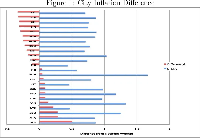
Figures 1 – 5 show the differences which exist across cities. All the data presented is the average over the period 2000-2008. Figure 1 shows the difference between city j, and the national average of inflation, ¯πj−π¯U S and the

standard deviation of this difference as a measure of inflation differential volatility. As can be clearly seen, there is about a one-percent difference between the highest inflation city (Seattle) and the lowest one (St. Louis). The average difference between the highest and lowest inflation cities over the sample period was about 5%. A word of caution: this does not mean that Seattle and St. Louis have the highest and lowest price levels

[image:5.612.144.469.271.494.2]

over the period, simply price changes. Looking at this data it appears the national inflation average is closest to Philadelphia. All data have been seasonally adjusted.

Figure 1: City Inflation Difference

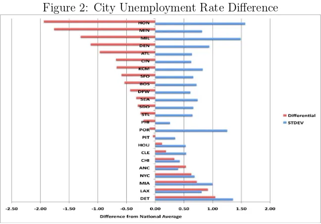
Figure 2 shows the same for unemployment rates across US cities: ¯uj−u¯U S. Given

frictions in individual labor markets we can see there is a considerable difference be-tween the highest unemployment city (Detroit) and the lowest (Honolulu), about 3%. The average difference between the highest and lowest unemployment cities over the sample period was about 5%. Visually, it appears the national average is closest to Pittsburgh. As might be expected, cities with the most volatility are those with largest unemployment difference. It is interesting to note Portland’s unemployment standard deviation, which is quite high. Generally, Portland’s unemployment is very close to the US as a whole; however, the recession of 2001 hit Portland particularly hard, and its unemployment rose two percentage points above the nation’s in 2002-03.

1

(6)

[image:6.612.144.468.79.305.2]

Figure 2: City Unemployment Rate Difference

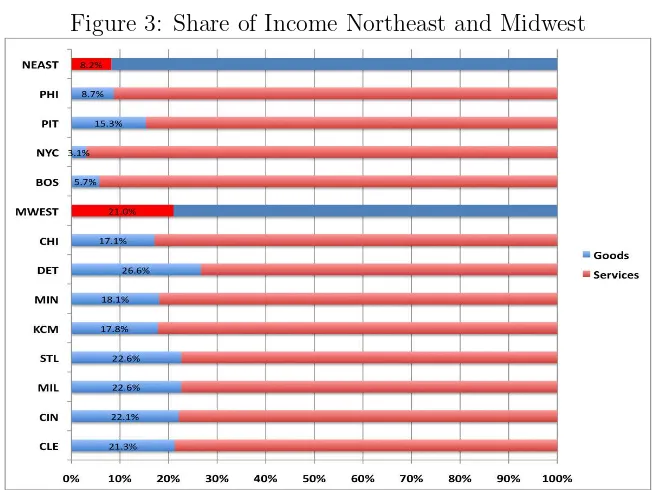
Now we turn our attention to the composition of production. Figures 3 and 4 show the output shares forprivategoods and services, percentages shown are the goods share, for the Northeast and Midwest, Figure 3, and the South and West, Figure 4 – the regions are split into the Bureau of Labor Statistics (BLS) regions, for the period 2001-2008.2 We also show the average for each region. The goods average for the Northeast and Midwest are about 21.0% and 8.2% respectively. Considering the South and West in Figure 4 the service goods are almost the same 16.7% and 16.8%. Unsurprisingly, given industry and agriculture, the Midwest produces the highest percentage of goods. We also see considerable differences between cities, even within the same state; for example, in San Francisco the goods share is almost under six percent, while in San Diego it is 22.5%.

Figure 5 shows the percentage difference of the goods share of each city (actual data is at the county level) vis-´a-vis the US average: ln(yServices

j /yU SServices) for the period

2001 – 08.3

As can be seen, the majority of cities produces less goods than the US, with the closest cities to the national average being Houston and St. Louis. What is also striking is that the majority of large US cities produce less than the national average – the national average isfor allcities, not just the cities in our sample. The theory below provides a model to understand why monetary policy may have differential effects.

3 Theory

Consider an international version of a New Keynesian business-cycle model. Rather than look at the propagation of business cycles across nations, we examine a “city-state” rendering of the model, with a home city and all others. We assume that each

2

The BLS adopted the North American Industry Classification System (NAICS) for classifying business types and started presenting business classifications in 2001, hence, for this comparison, we rely on data from 2001 on. The BLS regions are used because the price and income per capita data come from BLS.

3

(7)

[image:7.612.142.469.75.320.2]

Figure 3: Share of Income Northeast and Midwest

city is ‘small’ and it trades with all other cities which combined become as a homogenous ‘foreign’ city. For any variable xt, we will denote home city, denoted j, variables as

xt = xj,t and foreign variables x∗t = x−_j,t, that is all cities other than j. Because

the home city is small, x∗

t can be understood as the ‘national average’ of variable

x. Another assumption of such an economy is perfect capital mobility, such that the

nominalinterest rate will be the same across all city-states. What is also implied is that residents of city states are citizens of a single nation and, therefore, put their savings in a single instrument, say a federal government bond.

A conclusion we can draw from the data is that a number of ‘small open macroe-conomies’ exist, each with its own idiosyncratic, macroeconomic fluctuations. We em-ploy a New Keynesian model based on Clarida, Gal´ı and Gertner (2001). Domestic household consumption, ct, is a CES composite of home and foreign produced goods

ct= (1−γ)cht +γc f

t, γ ≥0 (1)

where ch t(c

f

t) is the amount of domestic consumption of home (foreign, or imported)

produced goods andγis a measure of openness, or as the percentage of foreign-produced goods in the domestic consumption basket. We can think of domestically-produced goods as non-traded goods and services, nationwide the percentage of services in the household expenditures is about 65%.

Domestic output is divided between home and foreign consumption of domestic goods,ch∗

t , or

yt= (1−γ)cht +γch

∗

t . (2)

The household maximizes its intertemporal utility, a function of the composite con-sumption good and leisure, ℓt,

U =Et T

X

t=0

(8)

[image:8.612.141.469.76.321.2]

Figure 4: Share of Income South and West

subject to an appropriate budget constraint. In this model, an implicit assumption is perfect intercity risk-sharing, a fair assumption as all the ‘countries’ are in a single currency area. We have the first-order conditions, in log-linear form,

cht −c f

t =ηqt, (4)

wt−pt−γqt= (φnt+σct) +µw, (5)

∆ce_t+1 = 1

σ[(i

∗

t −πte+1) +ρ−∆qet+1)] (6) and

∆q_te+1 = (i ∗

t −πte+1)−(i ∗

t −π

∗e

t+1) (7)

where for any variablext, xet+1 =Etxt+1;ρ= lnβ; andqt=p∗t−ptis the relative price

of the home to foreign cities price levels. 4

Equation (4) is the marginal rate of substitution between domestic and foreign produced goods whereηis the elasticity of substitution. Equation (5) is the relationship between the real wage and the marginal rate of substitution for consumption and labor, where nt = 1−ℓt is labor, φ is the inverse of labor supply elasticity, σ is the risk

aversion parameter, and µw _{is a wage friction, or mark-up (for example, long term}

wage contracts) which distorts the wage from its long-run equilibrium.

Equation (6) is a standard Euler equation, which shows the relationship between consumption and returns to savings. We think of this in terms of returns to home bonds, which is given by the expected real interest rate,re

t =i

∗

t−πte+1, under the assumption of perfect capital and asset mobility,it=i∗t, the city nominal interest rates are equal.

Note, however, because πt 6= π∗t the real interest rate across cities differs, which will

4

(9)

[image:9.612.116.500.81.420.2]

Figure 5: Share of City Goods Income Relative to National Average

affect consumption behavior across cities according to equation (6). Finally, equation (7), is a version of the terms of trade, uncovered interest parity condition. Nominal interest rates remain for the time being to remind the reader that real interest rates vary across cities. We assume that, under assumptions of risk sharing and the stationarity of shocks in the long run, that intercity PPP holds such that limt→∞q_t→ Q 6= 0, see

Footnote 4 above, and thus equation (7) holds. The city ‘real exchange rate’ or terms of trade – this result comes from the fact that the implicit exchange rate between all cities is one.

Next, we turn our attention to foreign demand for home-traded goods. Given that the rest of the country is large relative to each city, the home city’s share of production exported is negligible. From Gal´ı and Monacelli (2005) we assume that, for all other cities, output is equal to domestic consumption, y∗

= c∗

and national inflation, that is not influenced by the home city’s rate of inflation. The foreign demand for home production depends on foreign output and the terms of trade

ch∗

t =y

∗

t +ηqt. (8)

(10)

rate is proportional to output growth

i∗

t −π

∗_e

t+1=σ(y ∗

t+1−y ∗

t) (9)

where national output growth is taken to be exogenous to a specific city’s economic activity.

We consider a linear production function for all goods that is homogeneous of degree one in labor only

yt=at+nt, (10)

at is a productivity shock. With monopolistic, price-setting behavior, each city’s firms

base their pricing behavior on expected price changes and marginal cost. In the aggre-gate, the overall inflation rate is derived from a modified New Keynesian Phillips curve (NKPC) as

πt=zπ∗t+1e +δ(wt−pt−at) (11)

where the term in parenthesis is the marginal cost of production, derived from cost minimization. The textbook version of the NKPC uses the output gap, however Gal´ı and Monacelli (2005) demonstrate that substituting marginal cost for the gap has better empirical success. Note that city firms base their pricing behavior on the national average inflation rate rather than city-specific ones. Because of the high degree of mobility for consumption goods, firms are less willing to put their prices at a competitive disadvantage with other city firms. However, each city faces different labor markets; therefore, the marginal cost of production varies across cities resulting in idiosyncratic inflation rates.

Define ¯x to be thesteady-state or equilibrium level of variablex. Specifically, let ¯y

be the natural rate of output, ˆy =y−y¯is the output gap. We can solve the model as:

ˆ

yt = ˆyte+1− 1 +θ

σ (r

e

t+1−r¯t) +ζt (12)

πt = zπt∗+1e +λθyˆt+ut (13)

qt =

σ

1 +θyˆt+ ¯qt (14)

where θ = γ(ση−1)(2−γ); α = (σ/(1 +θ+φ); λθ = αδ and ut = δµwt; and ζt is

a stationary demand shock which can be decomposed into city-specific and national components: ζt = ζj,t +sjζt∗, sj is a measure of city j’s idiosyncratic response to a

nationwide shock. The steady states are given by:

¯

yt = α[(1 +φ)at−σθκyt∗]

¯

rt = θκrt∗+σκ(¯yte+1−y¯t)

¯

qt = σκ(¯yt−yt∗)

withκ= (1 +θ)−1_.

(11)

Equation (14) states that a city’s terms of trade are positively related to the output gap and the long-run terms of trade. We might also expect that city relative prices should converge in the long run, that is ¯qt = 0, but we can see that the steady-state

terms of trade is not equal to zero. In the intercity relative price literature, there is considerable evidence showing persistent differences in city-specific terms of trade (e.g. Cecchetti, Mark, and Sonora, 2002). Indeed, this equation resembles Kravis and Lipsey (1983) demand function – persistent price differences can be explained by city-specific productivity differences or income and preference differences, and thus relative prices converge to some non-zero mean.

3.1 Policy Rule

To close the model, we need to consider some interest rate or monetary policy rule. The standard way is to identify a monetary loss function based on some relationship between inflation and the output gap (or unemployment). With differences in city relative prices, or terms of trade, policy differs from a single, closed-economy model. However, as the terms of trade in equation (14) are proportional to the output gap, the policy objective can be written in the standard loss function form.

We begin with the assumption that each city loss function differs due to idiosyn-cratic macroeconomic conditions. For example, Detroit may be willing to take on more inflation to reduce its above-average unemployment while high inflation cities such as Seattle, would prefer the opposite. Thus, there exists tension between these two cities if the federal monetary authority favors one city over the other.

Hefeker (2003) considers such a case. Define the period, city-specific loss function as

L=b(nt−n¯t)2+π2t, b >0 (15)

where ¯n is the natural rate of employment, or, alternatively, an employment target, and breflects the city central bank’s preferences. Let employment be driven by

nt=c(πt−πte+1) +ǫ+dξ ∗

(16)

thus, employment, in the short run can be driven by inflationary surprises if wages are fixed for a period. ǫis a city-specific, idiosyncratic shock, andξ∗

is a nationwide shock,

d >0 measures the city’s idiosyncratic response to that national shock.

With a single monetary authority, the central bank minimizes the nationwide analog to equation (15) as

L∗

=b∗

(n∗

t −n¯

∗

t)

2 +π∗2

t , b

∗

>0, (17) similarly

n∗

t =c

∗

(π∗

t −π

∗e

t+1) + ¯ǫ+ξ ∗

(18)

where ¯ǫ=Pk

hjǫ, ¯n∗ =Pkhjn,¯ Phj = 1 for the kcities, hj <1 is relative weight of

each city, and Pk

hj = 1.

Minimizing equation(15) subject to (16) we get optimal inflation in thejth _city

π = Γ[¯n−(ǫ+dξ∗

)] (19)

(12)

monetary authority is made based on the median governor, therefore the country’s optimal inflation is determined by this policy maker,

πm= Γm[¯nm−(ǫm+dmξ∗)] (20)

where the m subscript denotes the median outcome with the associated preferences. Combining equations (19) and (20) with (15) we get a city specific welfare loss of a decision made by the median policy maker

L(M) =bi[(Γ−1)¯n+ (1−c)(ǫ+dξ

∗

)]2 +¡

Γm[¯nm−(ǫm+dmξ

∗

)]¢2

(21)

where L(M) is the city loss function associated with the decision made by the me-dian governor. Thus, the individual city loss function differs from the one employed nationally and thus implies a suboptimal, to the city, Taylor rule.

If each city were to design a Taylor rule, say,

rt= ¯r+fj(πt−π¯tτ) + ˆyt, (22)

fj is the city bank’s inflation weight and ¯πτ is the countrywide inflation target, and

compare this to a similarly constructed median (central bank’s) governor’s Taylor rule

rm,t = ¯r+fm(π

∗

t −π¯τt) + ˆy

∗

t (23)

we would see a difference in the policy interest rate as

rt=rm,t+χt, (24)

whereχt= (fjπt−fmπt∗) + (ˆyt−yˆt∗) is a suboptimal policy premium. Note, even if city

preferences were identical to the central bank’s preferences, f ≡ fi = fm, the policy

interest premium would still differ across cities because of heterogeneous inflation and output gaps, with χt 6= 0. Under the assumption fi = fm, combining equations (12)

and (24) we get the city aggregate demand curve

ˆ

yt=δ′+ (1−δ)yte+1−δf(πte+1−π ∗e

t+1) +ψt (25)

withδ′

=−δre

m,t+1 and ψt=δy ∗e t+1+ζt.

4 Empirical Methodology

The major metropolitan areas identified above have data available to investigate the hypothesis that U.S. cities experience differential effects from monetary policy. Mon-etary policy should have effects on income per capita, prices and unemployment that differ from city to city5

. Cities are used to not only complement the effects shown in Carlino and Defina (1998, 1999) that interest-sensitive regions of the United States face larger effects of monetary policy than other regions, but introduce data on inflation into this regional policy literature.

5

(13)

4.1 Estimation Data and Variables

Turning our attention to city macroeconomic data, we can see the manifestation of these differences in income data, but also in unemployment and price data. The data we consider are semi-annual. City specific output data at a higher frequency is not available. All city data is from the Bureau of Labor Statistics (www.bls.gov) and in-cludes city-specific income per capita, unemployment, and prices. The federal funds data is from the Board of Governors of the Federal Reserve (www.federalreserve.gov). As previously suggested, considerable differences across cities exist; for a host of rea-sons, city-specific inflation, income per capita (as a proxy for city output levels) and unemployment experience heterogeneous responses to a single monetary shock with respect to the national reaction. Additionally, a change in monetary policy reflects a median governor which may benefit cities at the distribution’s center but hurt those in the tails.

Monetary policy is characterized by changes in the federal funds rate (ffr).6_{. These} monthly data are converted into a semi-annual series using a 6-month centered moving average. The data on unemployment rates are at the municipal level, which is also true for prices and income. These data are also converted to a semi-annual frequency; population was also found at the Bureau of Labor Statistics (BLS) to normalize income measurements to per-capita figures. This conversion reduces the possibility of spurious correlations based on the sheer size of large cities in comparison to small cities. All these series have potential nonstationarity in either their levels or their first differences for some subset of the municipalities. Because we are ultimately testing for deviations from the national movements in these variables, the data on prices, unemployment and income per capita are made into a ratio with their national counterpart. For each home city j in our data, the variables are as follows:

Pj =

Pj

PU S

; and Uj =

Uj

UU S

; and W P Cj =

(Inc/Cap)j

(Inc/Cap)U S

The labeling in the results below needs some explanation. For example, the variable PANC refers to the ratio of the inflation rates in Anchorage, Alaska to the U.S. inflation rate for urban areas. UANC and WPCANC are the example variables for Anchorage for unemployment and income per capita respectively. Each city’s ratios with the national level are stationary for all data at the 5% level of both Phillip-Perron and Augmented Dickey-Fuller (ADF) tests.

We assume a change inffr is exogenous to the determination of the other variables. The figures below describe how the path of these ratios change when monetary policy takes place. In this study, there are four variables, 24 cities, and 38 observations of each variable for city i from 1990 to 2008.

4.2 Vector Autoregressions

Vector Autoregressions (VARs) are a standard econometric method used when test-ing hypotheses concerntest-ing policy effects on macroeconomic variables. Similar to error correction models, VARs regress a vector of variables at time t on the same vector of

6

(14)

variables with a distributed lag structure and perhaps other variables assumed to be exogenous to the vector of focal variables. The lag structure is determined by informa-tion criteria, where the Akaike and Schwarz Criteria are examples. The error term in such an estimation is considered to be a vector of uncorrelated, zero-mean innovations to the variables within the original vector. Such a model allows for an impulse response analysis by simulating a change in one variable’s disturbances and examining how that would change the relationships among the other variables through a distributed lag. The AS and AD equations, (13) and (25), formalize the VAR analysis. Equation (26) describes the vector of variables for this study; in this analysis, we study the dynamic behavior of 24 metropolitan-level vectors, assumed to be covariance stationary, with six variables each.

Y_i,t _{= (}_{f f r}_t_{, P}_i,t_{, U}_i,t_{, W P C}_i,t_,Z_t₎ ₍₂₆₎

The index t is time and i represents the index over the 24 cities in our sample. Z

represents a vector of other, exogenous variables. Following Carlino and Defina’s (1998, 1999) studies, the use of the leading indicator from the Conference Board (LEAD) and the Bureau of Labor Statistics’ producer price index for fuel prices (PPIFUELS) as exogenous variables provides aggregate demand (LEAD) and supply (PPIFUELS) variables for identification. The VAR and the dynamics of our choice variables are described in equation (27).

AY_i,t₌B₍_L₎Y_i,t−p+εi,t (27)

In equation (27), A _{is a (6}×6) matrix of correlation coefficients for the variables in

Y_; B _{is a (6}_×_{6) matrix represents the polynomial relationships describing the lag}

operator L and ε is the vector of disturbances. We restrict the variance-covariance matrix to force the exogenous variables LEAD and PPIFUELS to be exogenous and have no contemporaneous correlations. In the reduced form model, the disturbances would be converted toυ, which is simply the product of the inverse of theA_{matrix in}

equation (26) and the structural disturbances, ε.

5 Results

5.1 Impulse Response Functions

VARs recognize the relationship between past and current values of the same variables and the potential for bidirectional causality7

. For example, monetary policy may both cause and be caused by changes in income, inflation or unemployment. In our model, we assume that current and lagged values of the federal funds rate determine inflation, unemployment and income levels at the national and metropolitan levels. The VAR residuals allow us to analyze an impulse response function (IRF). In our model, the “impulse ”is a monetary policy change acting like an unanticipated shock; the response is how the three endogenous variables react to the specific impulse, a one standard-deviation increase in the federal funds rate. The IRF methodology implies that a rate

7

(15)

cut would simply be the mirror image of the increase8

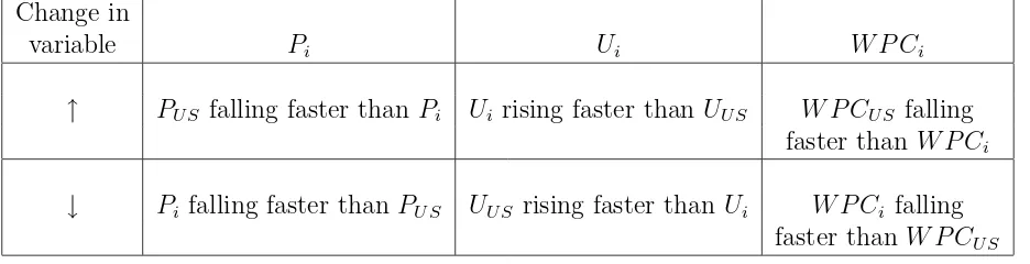
[image:15.612.70.538.148.268.2]

. Table 1 summarizes how to interpret the impulse responses.

Table 1: Impulse Response Summary: A one standard deviation increase in ffr Change in

variable P_i U_i W P C_i

↑ P_{U S} _{falling faster than} P_i U_i _{rising faster than} U_{U S} W P C_{U S} _falling faster than W P C_i

↓ P_i _{falling faster than} P_{U S} U_{U S} _{rising faster than} U_i W P C_i _falling faster than W P C_{U S}

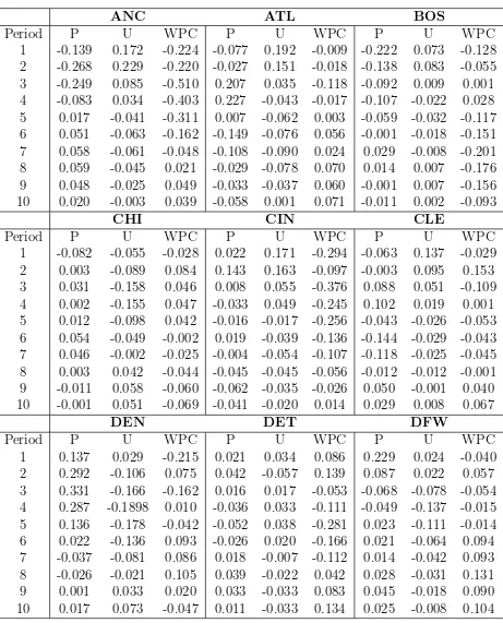
We begin by considering the period-by-period impulse response results for ten pe-riods (five years) in Tables 2 – 4. As can be seen, there is considerable heterogeneity of the responses across the cities. Moreover, the timing of the direction and speed of adjustment varies across the cities – and tends to cluster over the ten periods of impulse response. For example, consider Chicago in Table 2, the national average unemploy-ment rate rises faster following a shock, however, this is reversed after four years. The opposite trend occurs with respect to income, which is due to the Okun effect. On the other hand, prices generally rise faster in Chicago vis-´a-vis the overall CPI. Looking at Cincinnati, next to Chicago in the table, its income fallsevery period following the shock, except for period 10, while unemployment initially rises and then falls relative to the average. Also, a weaker negative relationship between unemployment and per capita income. From this side-by-side comparison, it appears Chicago fares better than Cincinnati following a monetary shock as a ”macroeconomy”.

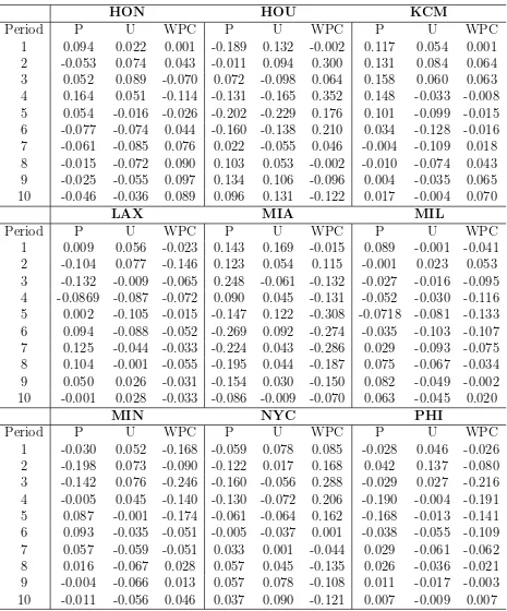
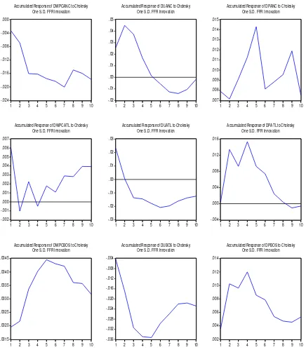
Next, consider the cumulative impulse responses shown in Figures 6 through 13. We should evaluate the results in terms of the differential effects of monetary policy across the United States. When there is a monetary shock, we would expect the included variables to react according to theory. For income per capita, we would expect an increase in the federal funds rate to reduce income growth; for inflation, we expect a slowdown also, and for unemployment we expect an increase. Because our variables are deviations from the national response, or how differently the home city’s reacts to a national monetary policy relative to the national reaction.

An example helps illustrate the results. In Figure 6, for example, the results for Atlanta (ATL) are in the middle row of 6. The monetary contraction initially increases prices more than the change in the national level, increases unemployment in net more than at the national level, and decreases wages versus the national level. After four or five time periods, two years after the initial shock, the regional change is more like the national change; the ratio converges or begins converging after ten periods. In contrast, Boston (BOS) in 6, does not converge in any of the variables. The monetary

8

(16)

[image:16.612.79.540.113.684.2]

Table 2: Impulse Responses to a one std dev change in ffr: Prices, Unemployment and Income/Capita

ANC

ATL

BOS

Period

P

U

WPC

P

U

WPC

P

U

WPC

1 -0.139

0.172 -0.224 -0.077

0.192 -0.009 -0.222

0.073 -0.128

2 -0.268

0.229 -0.220 -0.027

0.151 -0.018 -0.138

0.083 -0.055

3 -0.249

0.085 -0.510

0.207

0.035 -0.118 -0.092

0.009

0.001

4 -0.083

0.034 -0.403

0.227 -0.043 -0.017 -0.107 -0.022

0.028

5

0.017 -0.041

-0.311

0.007 -0.062

0.003 -0.059 -0.032 -0.117

6

0.051 -0.063

-0.162 -0.149 -0.076

0.056 -0.001 -0.018 -0.151

7

0.058 -0.061

-0.048 -0.108 -0.090

0.024

0.029 -0.008 -0.201

8

0.059 -0.045

0.021 -0.029 -0.078

0.070

0.014

0.007 -0.176

9

0.048 -0.025

0.049 -0.033 -0.037

0.060 -0.001

0.007 -0.156

10

0.020 -0.003

0.039 -0.058

0.001

0.071 -0.011

0.002 -0.093

CHI

CIN

CLE

Period

P

U

WPC

P

U

WPC

P

U

WPC

1 -0.082

-0.055

-0.028

0.022

0.171 -0.294 -0.063

0.137 -0.029

2

0.003 -0.089

0.084

0.143

0.163 -0.097 -0.003

0.095

0.153

3

0.031 -0.158

0.046

0.008

0.055 -0.376

0.088

0.051 -0.109

4

0.002 -0.155

0.047 -0.033

0.049 -0.245

0.102

0.019

0.001

5

0.012 -0.098

0.042 -0.016 -0.017 -0.256 -0.043 -0.026 -0.053

6

0.054 -0.049

-0.002

0.019 -0.039 -0.136 -0.144 -0.029 -0.043

7

0.046 -0.002

-0.025 -0.004 -0.054 -0.107 -0.118 -0.025 -0.045

8

0.003

0.042 -0.044 -0.045 -0.045 -0.056 -0.012 -0.012 -0.001

9 -0.011

0.058 -0.060 -0.062 -0.035 -0.026

0.050 -0.001

0.040

10 -0.001

0.051 -0.069 -0.041 -0.020

0.014

0.029

0.008

0.067 DEN

DET

DFW

Period

P

U

WPC

P

U

WPC

P

U

WPC

(17)

[image:17.612.78.543.115.675.2]

HON

HOU

KCM

Period

P

U

WPC

P

U

WPC

P

U

WPC

1

0.094

0.022

0.001 -0.189

0.132 -0.002

0.117

0.054

0.001

2 -0.053

0.074

0.043 -0.011

0.094

0.300

0.131

0.084

0.064

3

0.052

0.089 -0.070

0.072 -0.098

0.064

0.158

0.060

0.063

4

0.164

0.051 -0.114 -0.131 -0.165

0.352

0.148 -0.033 -0.008

5

0.054 -0.016 -0.026 -0.202 -0.229

0.176

0.101 -0.099 -0.015

6 -0.077

-0.074

0.044 -0.160 -0.138

0.210

0.034 -0.128 -0.016

7 -0.061

-0.085

0.076

0.022 -0.055

0.046 -0.004

-0.109

0.018

8 -0.015

-0.072

0.090

0.103

0.053 -0.002

-0.010

-0.074

0.043

9 -0.025

-0.055

0.097

0.134

0.106 -0.096

0.004 -0.035

0.065

10 -0.046

-0.036

0.089

0.096

0.131 -0.122

0.017 -0.004

0.070 LAX

MIA

MIL

Period

P

U

WPC

P

U

WPC

P

U

WPC

1

0.009

0.056 -0.023

0.143

0.169 -0.015

0.089 -0.001 -0.041

2 -0.104

0.077 -0.146

0.123

0.054

0.115 -0.001

0.023

0.053

3 -0.132

-0.009 -0.065

0.248 -0.061 -0.132

-0.027

-0.016 -0.095

4 -0.0869 -0.087 -0.072

0.090

0.045 -0.131

-0.052

-0.030 -0.116

5

0.002 -0.105 -0.015 -0.147

0.122 -0.308 -0.0718 -0.081 -0.133

6

0.094 -0.088 -0.052 -0.269

0.092 -0.274

-0.035

-0.103 -0.107

7

0.125 -0.044 -0.033 -0.224

0.043 -0.286

0.029 -0.093 -0.075

8

0.104 -0.001 -0.055 -0.195

0.044 -0.187

0.075 -0.067 -0.034

9

0.050

0.026 -0.031 -0.154

0.030 -0.150

0.082 -0.049 -0.002

10 -0.001

0.028 -0.033 -0.086 -0.009 -0.070

0.063 -0.045

0.020 MIN

NYC

PHI

Period

P

U

WPC

P

U

WPC

P

U

WPC

(18)

[image:18.612.77.544.116.493.2]

PIT

POR

SDO

Period

P

U

WPC

P

U

WPC

P

U

WPC

1

0.036

0.054 -0.098

0.140

0.013 -0.043 -0.050 -0.082

0.054

2

0.123

0.128 -0.035 -0.021

-0.140

0.241 -0.135 -0.233

0.099

3

0.082

0.017 -0.030 -0.027

-0.129

0.048 -0.234 -0.283

0.111

4 -0.042 -0.076 -0.005

0.086 -0.035

0.066 -0.202 -0.272

0.067

5 -0.088 -0.130 -0.028

0.122

0.009

0.010 -0.124 -0.206

0.024

6 -0.070 -0.136 -0.060

0.067

0.036

0.001 -0.065 -0.096

0.000

7 -0.036 -0.112 -0.056 -0.001

0.051 -0.051 -0.038

0.026

0.013

8 -0.010 -0.078 -0.021 -0.026

0.066 -0.078 -0.036

0.122

0.054

9

0.007 -0.041

0.015 -0.027

0.066 -0.093 -0.054

0.167

0.112

10

0.019 -0.005

0.038 -0.027

0.052 -0.088 -0.089

0.161

0.171 SEA

SFO

STL

Period

P

U

WPC

P

U

WPC

P

U

WPC

1 -0.070 -0.040

0.040 -0.057

0.06336

-0.094 -0.072

0.036 -0.053

2 -0.021 -0.082 -0.093 -0.009

0.07268

0.315 -0.003

0.083

0.021

3

0.191 -0.114 -0.252

0.208 -0.03289

0.254 -0.071

0.067

0.080

4

0.290 -0.157 -0.307

0.245 -0.03714 -0.064 -0.181

0.027

0.049

5

0.273 -0.190 -0.309

0.127 -0.02917 -0.298 -0.182 -0.021

0.073

6

0.202 -0.176 -0.271 -0.053 -0.00207 -0.312 -0.117 -0.067

0.175

7

0.120 -0.131 -0.232 -0.136 -0.00957 -0.213 -0.057 -0.093

0.206

8

0.055 -0.080 -0.203 -0.118 -0.02274 -0.115

0.005 -0.088

0.128

9

0.023 -0.040 -0.191 -0.038 -0.03971 -0.046

0.070 -0.065

0.024

10

0.016 -0.016 -0.186

0.043 -0.046

-0.011

0.108 -0.036 -0.058

contraction reduces prices in Boston more permanently as compared to the national level. Unemployment rises in a permanent fashion, and income per capita is also forced down permanently. Many of the other cities have relatively more temporary effects. There is evidence that monetary policy does not affect municipalities in similar ways, which corroborates Carlino and Defina’s (1998, 1999) studies concerning differential effects on income while adding the inflation relationship among the cities.

(19)

-.024 -.020 -.016 -.012 -.008 -.004 .000

1 2 3 4 5 6 7 8 9 10 Accumulated Response of DWPCANC to Cholesky

One S.D. FFR Innovation

-.02 -.01 .00 .01 .02 .03 .04 .05

1 2 3 4 5 6 7 8 9 10 Accumulated Response of DUANC to Cholesky

.007 .008 .009 .010 .011 .012 .013 .014 .015

1 2 3 4 5 6 7 8 9 10 Accumulated Response of DPANC to Cholesky

-.002 -.001 .000 .001 .002 .003 .004 .005 .006 .007

1 2 3 4 5 6 7 8 9 10 Accumulated Response of DWPCATL to Cholesky

-.03 -.02 -.01 .00 .01 .02 .03

1 2 3 4 5 6 7 8 9 10 Accumulated Response of DUATL to Cholesky

-.004 .000 .004 .008 .012 .016

1 2 3 4 5 6 7 8 9 10 Accumulated Response of DPATL to Cholesky

.0015 .0020 .0025 .0030 .0035 .0040 .0045

1 2 3 4 5 6 7 8 9 10 Accumulated Response of DWPCBOS to Cholesky

-.036 -.032 -.028 -.024 -.020 -.016 -.012 -.008 -.004

1 2 3 4 5 6 7 8 9 10 Accumulated Response of DUBOS to Cholesky

.002 .004 .006 .008 .010 .012 .014

1 2 3 4 5 6 7 8 9 10 Accumulated Response of DPBOS to Cholesky

[image:19.612.89.525.125.627.2]

(20)

-.004 -.003 -.002 -.001 .000 .001

1 2 3 4 5 6 7 8 9 10 Accumulated Response of DWPCCHI to Cholesky

-.016 -.012 -.008 -.004 .000 .004

1 2 3 4 5 6 7 8 9 10 Accumulated Response of DUCHI to Cholesky

-.002 -.001 .000 .001 .002 .003 .004 .005 .006 .007

1 2 3 4 5 6 7 8 9 10 Accumulated Response of DPCHI to Cholesky

-.012 -.008 -.004 .000 .004 .008

1 2 3 4 5 6 7 8 9 10 Accumulated Response of DWPCCIN to Cholesky

-.020 -.015 -.010 -.005 .000 .005 .010 .015

1 2 3 4 5 6 7 8 9 10 Accumulated Response of DUCIN to Cholesky

-.006 -.004 -.002 .000 .002 .004 .006

1 2 3 4 5 6 7 8 9 10 Accumulated Response of DPCIN to Cholesky

-.007 -.006 -.005 -.004 -.003 -.002 -.001 .000 .001 .002

1 2 3 4 5 6 7 8 9 10 Accumulated Response of DWPCCLE to Cholesky

-.03 -.02 -.01 .00 .01 .02

1 2 3 4 5 6 7 8 9 10 Accumulated Response of DUCLE to Cholesky

.000 .002 .004 .006 .008 .010 .012 .014 .016

1 2 3 4 5 6 7 8 9 10 Accumulated Response of DPCLE to Cholesky

[image:20.612.88.521.129.627.2]

(21)

-.003 -.002 -.001 .000 .001 .002 .003 .004

1 2 3 4 5 6 7 8 9 10 Accumulated Response of DWPCDEN to Cholesky

-.020 -.015 -.010 -.005 .000 .005 .010

1 2 3 4 5 6 7 8 9 10 Accumulated Response of DUDEN to Cholesky

-.012 -.008 -.004 .000 .004 .008

1 2 3 4 5 6 7 8 9 10 Accumulated Response of DPDEN to Cholesky

-.012 -.010 -.008 -.006 -.004 -.002 .000

1 2 3 4 5 6 7 8 9 10 Accumulated Response of DWPCDET to Cholesky

-.05 -.04 -.03 -.02 -.01 .00

1 2 3 4 5 6 7 8 9 10 Accumulated Response of DUDET to Cholesky

.000 .004 .008 .012 .016 .020

1 2 3 4 5 6 7 8 9 10 Accumulated Response of DPDET to Cholesky

-.002 .000 .002 .004 .006 .008 .010 .012 .014

1 2 3 4 5 6 7 8 9 10 Accumulated Response of DWPCDFW to Cholesky

-.032 -.028 -.024 -.020 -.016 -.012 -.008 -.004

1 2 3 4 5 6 7 8 9 10 Accumulated Response of DUDFW to Cholesky

-.012 -.010 -.008 -.006 -.004 -.002 .000

1 2 3 4 5 6 7 8 9 10 Accumulated Response of DPDFW to Cholesky

[image:21.612.88.522.129.631.2]

(22)

-.010 -.008 -.006 -.004 -.002 .000 .002

1 2 3 4 5 6 7 8 9 10 Accumulated Response of DWPCHON to Cholesky

.016 .020 .024 .028 .032 .036 .040 .044 .048 .052

1 2 3 4 5 6 7 8 9 10 Accumulated Response of DUHON to Cholesky

-.004 .000 .004 .008 .012 .016

1 2 3 4 5 6 7 8 9 10 Accumulated Response of DPHON to Cholesky

-.004 -.002 .000 .002 .004 .006 .008 .010 .012

1 2 3 4 5 6 7 8 9 10 Accumulated Response of DWPCHOU to Cholesky

-.05 -.04 -.03 -.02 -.01 .00 .01 .02 .03

1 2 3 4 5 6 7 8 9 10 Accumulated Response of DUHOU to Cholesky

.006 .007 .008 .009 .010 .011 .012 .013 .014

1 2 3 4 5 6 7 8 9 10 Accumulated Response of DPHOU to Cholesky

-.004 -.002 .000 .002 .004 .006 .008

1 2 3 4 5 6 7 8 9 10 Accumulated Response of DWPCKCM to Cholesky

-.05 -.04 -.03 -.02 -.01 .00 .01

1 2 3 4 5 6 7 8 9 10 Accumulated Response of DUKCM to Cholesky

-.012 -.008 -.004 .000 .004 .008

1 2 3 4 5 6 7 8 9 10 Accumulated Response of DPKCM to Cholesky

[image:22.612.90.522.129.623.2]

(23)

-.009 -.008 -.007 -.006 -.005 -.004 -.003 -.002 -.001

1 2 3 4 5 6 7 8 9 10 Accumulated Response of DWPCLAX to Cholesky

.00 .01 .02 .03 .04 .05

1 2 3 4 5 6 7 8 9 10 Accumulated Response of DULAX to Cholesky

-.012 -.008 -.004 .000 .004 .008

1 2 3 4 5 6 7 8 9 10 Accumulated Response of DPLAX to Cholesky

-.014 -.012 -.010 -.008 -.006 -.004 -.002

1 2 3 4 5 6 7 8 9 10 Accumulated Response of DWPCMIA to Cholesky

.00 .01 .02 .03 .04 .05

1 2 3 4 5 6 7 8 9 10 Accumulated Response of DUMIA to Cholesky

.002 .003 .004 .005 .006 .007 .008 .009

1 2 3 4 5 6 7 8 9 10 Accumulated Response of DPMIA to Cholesky

-.008 -.007 -.006 -.005 -.004 -.003 -.002 -.001 .000

1 2 3 4 5 6 7 8 9 10 Accumulated Response of DWPCMIL to Cholesky

-.02 -.01 .00 .01 .02 .03

1 2 3 4 5 6 7 8 9 10 Accumulated Response of DUMIL to Cholesky

.000 .002 .004 .006 .008 .010

1 2 3 4 5 6 7 8 9 10 Accumulated Response of DPMIL to Cholesky

[image:23.612.90.525.124.630.2]

(24)

-.006 -.005 -.004 -.003 -.002 -.001 .000

1 2 3 4 5 6 7 8 9 10 Accumulated Response of DWPCMIN to Cholesky

-.004 .000 .004 .008 .012 .016 .020 .024

1 2 3 4 5 6 7 8 9 10 Accumulated Response of DUMIN to Cholesky

-.004 .000 .004 .008 .012 .016 .020

1 2 3 4 5 6 7 8 9 10 Accumulated Response of DPMIN to Cholesky

-.012 -.008 -.004 .000 .004 .008 .012

1 2 3 4 5 6 7 8 9 10 Accumulated Response of DWPCNYC to Cholesky

-.005 .000 .005 .010 .015 .020 .025 .030

1 2 3 4 5 6 7 8 9 10 Accumulated Response of DUNYC to Cholesky

-.006 -.004 -.002 .000 .002 .004 .006

1 2 3 4 5 6 7 8 9 10 Accumulated Response of DPNYC to Cholesky

-.008 -.007 -.006 -.005 -.004 -.003 -.002 -.001 .000

1 2 3 4 5 6 7 8 9 10 Accumulated Response of DWPCPHI to Cholesky

-.010 -.005 .000 .005 .010 .015 .020

1 2 3 4 5 6 7 8 9 10 Accumulated Response of DUPHI to Cholesky

.000 .001 .002 .003 .004 .005 .006 .007 .008

1 2 3 4 5 6 7 8 9 10 Accumulated Response of DPPHI to Cholesky

[image:24.612.86.525.131.626.2]

(25)

-.008 -.006 -.004 -.002 .000 .002

1 2 3 4 5 6 7 8 9 10 Accumulated Response of DWPCPIT to Cholesky

-.03 -.02 -.01 .00 .01

1 2 3 4 5 6 7 8 9 10 Accumulated Response of DUPIT to Cholesky

.003 .004 .005 .006 .007 .008 .009

1 2 3 4 5 6 7 8 9 10 Accumulated Response of DPPIT to Cholesky

.000 .001 .002 .003 .004 .005 .006

1 2 3 4 5 6 7 8 9 10 Accumulated Response of DWPCPOR to Cholesky

-.02 -.01 .00 .01 .02 .03 .04

1 2 3 4 5 6 7 8 9 10 Accumulated Response of DUPOR to Cholesky

.000 .004 .008 .012 .016 .020

1 2 3 4 5 6 7 8 9 10 Accumulated Response of DPPOR to Cholesky

-.010 -.008 -.006 -.004 -.002 .000 .002 .004 .006

1 2 3 4 5 6 7 8 9 10 Accumulated Response of DWPCSDO to Cholesky

-.05 -.04 -.03 -.02 -.01 .00 .01 .02

1 2 3 4 5 6 7 8 9 10 Accumulated Response of DUSDO to Cholesky

.0020 .0025 .0030 .0035 .0040 .0045 .0050

1 2 3 4 5 6 7 8 9 10 Accumulated Response of DPSDO to Cholesky

[image:25.612.89.521.127.631.2]

(26)

-.016 -.012 -.008 -.004 .000 .004 .008 .012

1 2 3 4 5 6 7 8 9 10 Accumulated Response of DWPCSEA to Cholesky

-.006 -.004 -.002 .000 .002 .004 .006 .008

1 2 3 4 5 6 7 8 9 10 Accumulated Response of DUSEA to Cholesky

-.010 -.008 -.006 -.004 -.002 .000 .002 .004 .006

1 2 3 4 5 6 7 8 9 10 Accumulated Response of DPSEA to Cholesky

.000 .002 .004 .006 .008 .010 .012 .014

1 2 3 4 5 6 7 8 9 10 Accumulated Response of DWPCSFO to Cholesky

-.010 -.005 .000 .005 .010 .015 .020

1 2 3 4 5 6 7 8 9 10 Accumulated Response of DUSFO to Cholesky

-.004 .000 .004 .008 .012 .016 .020

1 2 3 4 5 6 7 8 9 10 Accumulated Response of DPSFO to Cholesky

-.20 -.16 -.12 -.08 -.04 .00 .04 .08

1 2 3 4 5 6 7 8 9 10 Accumulated Response of DWPCSTL to Cholesky

-.030 -.025 -.020 -.015 -.010 -.005 .000 .005 .010

1 2 3 4 5 6 7 8 9 10 Accumulated Response of DUSTL to Cholesky

-.02 -.01 .00 .01 .02 .03 .04

1 2 3 4 5 6 7 8 9 10 Accumulated Response of DPSTL to Cholesky

[image:26.612.90.522.125.636.2]

(27)

may provide ways for local areas to gauge the timing and magnitude of monetary policy locally.

The implications of AS curvature differences are that some areas receive different benefits from monetary policy in terms of job growth without inflation than others; as a corollary, some areas receive more inflation without the benefits of job growth. The relationship between price changes and unemployment changes as a result of policy is an easy way to make conclusions about AS curvature and how different cities may have flatter or steep curvatures. Evidence of a flatter AS curve would be price changes that were temporary and unemployment changes that were more permanent. This is shown in the impulse responses of such cities as CLE, CIN, HON, HOU, LAX, and PIT.

Other cities, such as ANC, BOS, DET, KCM, MIN, NYC, PHI, POR, SFO, and STL show more inflation than change in unemployment. The remaining cities are a mix of reactions. As an example, ATL shows no permanent effects on either prices or unemployment after a monetary policy shock. SDO shows a change consistent with a supply-side expansion, where prices and unemployment are both falling as the money supply contracts; CHI, DEN, and DFW show a stagflation-like effect as a result of a monetary contraction, where prices and unemployment rise at the same time. The explanation for why these differences exist is vast. As in Carlino and Defina (1998, 1999), differences in policy channel and interest rate sensitivities provide answers; Flo-rio (2005) updates Barro (1977, 1978) and suggests that aggregate supply differences provide evidence for differential effects. It is important that policy makers consider these explanations, especially if the Euro area intends to add more member nations in the wake of Greece’s debt crisis and the possible problems of other, ”regional” economies.

5.2 Correlation and Comparisons

(28)

[image:28.612.55.731.113.545.2]

Table 5: Correlations between Cities and Cumulative Responses to Policy: Income/Capita

(r >0.8 in absolute value, (City) represents negative correlation)

ANC ATL

BOS

CHI

CIN

CLE DEN

DET DFW HON HOU KCM LAX MIA MIL MIN NYC PHI

PIT POR SDO SEA SFO STL

(BOS)

CHI

CIN

CLE

(DEN) (DEN) (DEN)

(DET)

DET

(DFW)

DFW

(HOU)

HOU

(HOU) HOU

KCM KCM

MIA

(MIA)

MIL

MIN

(MIN)

MIN

PHI

PHI (PHI)

PHI

PIT

(PIT)

PIT

(SDO)

(SFO) (SFO)

(SFO)

SFO

(SFO)

STL

(29)

[image:29.612.57.736.112.544.2]

Table 6: Correlations between Cities and Cumulative Responses to Policy: Unemployment

ANC ATL BOS CHI CIN CLE DEN DET DFW

HON HOU KCM LAX MIA

MIL

MIN NYC

PHI

PIT POR SDO SEA SFO STL

BOS

CIN CIN

CLE CLE

CLE

DEN DEN

DFW

(HON)

HOU HOU

HOU HOU HOU

KCM

KCM (KCM)

(LAX)

LAX

(LAX)

(MIA)

MIA

(MIA) MIA

MIL

MIL (MIL)

MIL (MIL) (MIL)

MIN (MIN)

(MIN)

NYC

(NYC)

PHI

PHI (PHI)

PHI

(PHI)

PHI

PIT

PIT PIT

(PIT)

PIT

(PIT)

PIT

(POR)

POR (POR)

(POR) (POR)

(SDO)

SDO

(SDO)

(SDO) SDO SDO (SDO)

(SDO) (SDO) SDO

(SFO)

SFO

SFO (SFO)

(SFO)

SFO SFO (SFO) (SFO) SFO

SFO SFO

(STL)

(30)

[image:30.612.65.737.113.545.2]

Table 7: Correlations between Cities and Cumulative Responses to Policy: Inflation

ANC ATL BOS CHI CIN CLE DEN DET DFW HON HOU KCM LAX MIA MIL MIN NYC PHI PIT POR SDO SEA SFO STL

BOS

CLE CLE

DEN

DET DET

DET

DFW

HON HON

HON HON HON

HOU

KCM

LAX

MIL MIL

MIL

MIL MIL

MIL

MIN MIN

MIN MIN MIN

MIN

NYC

NYC NYC

NYC

PHI PHI

PHI PHI PHI

PHI PHI

PHI PHI PHI

PIT

POR

POR POR

SEA

SEA SEA

SEA

SFO SFO

SFO SFO SFO

SFO

SFO SFO

SFO SFO SFO

SFO

STL

(31)

6 Conclusions and Discussion

The United States as an optimal currency area is at the heart of this study. Our results suggest that monetary policy in the United States affects municipalities in a differential manner. Using VARs to identify the parameters and impulse response functions to estimate policy effects, this study used the ratio of consumer prices, unemployment and per capita income in 24 cities to the national average or totals to track how different certain cities were to others in their reactions to policy.

Because different municipalities react in different ways concerning prices and un-employment after a monetary shock, using a national model of aggregate supply to estimate policy effects may be erroneous. Further, policy makers may want to consider using a disaggregated model of monetary shocks and aggregate the effects. These results complement studies such as Carlino and Defina (1998, 1999) by expanding their conclu-sions to the aggregate supply curve concerning differential regional effects of monetary policy. We can expand these results by finding more home cities with price, unemploy-ment and income data; most counties have all but prices, and it is in local inflation where we likely learn the most about differential effects.

(32)

References

[1] R. J. Barro. Unanticipated money growth and unemployment in the united states.

The American Economic Review, 67(2):101–115, 1977.

[2] R. J. Barro. Unanticipated money, output, and the price level in the united states.

The Journal of Political Economy, 86(4):549–580, 1978.

[3] G. Carlino and R. Defina. The differential regional effects of monetary policy. The Review of Economics and Statistics, 80(4):572–587, November 1998.

[4] G. Carlino and R. DeFina. Do states respond differently to changes in monetary policy? Business Review, (Jul):17–27, 1999.

[5] S. G. Cecchetti, N. C. Mark, and R. J. Sonora. Price index convergence among united states cities. International Economic Review, 43(4):1081–1099, 2002.

[6] R. Clarida, J. Gal´ı, and M. Gertler. Optimal monetary policy in open versus closed economies: An integrated approach. The American Economic Review, 91(2):248– 252, 2001.

[7] J. P. Cover. Asymmetric effects of positive and negative money-supply shocks.

The Quarterly Journal of Economics, 107(4):1261–82, November 1992.

[8] A. Florio. Asymmetric monetary policy: empirical evidence for italy. Applied Economics, 37(7):751–764, April 2005.

[9] J. Gal´ı and T. Monacelli. Monetary policy and exchange rate volatility in a small open economy. The Review of Economic Studies, 72(3):707–734, 2005.

[10] W. H. Greene. Econometric Analysis (5th Edition). Prentice Hall, 2002.

[11] C. Hefeker. Federal monetary policy. The Scandinavian Journal of Economics, 105.

[12] O. Jorda. Estimation and inference of impulse responses by local projections.

American Economic Review, 95(1):161–182, March 2005.

[13] G. Karras. Are the output effects of monetary policy asymmetric? evidence from a sample of european countries. Oxford Bulletin of Economics and Statistics, 58(2):267–78, May 1996.

[14] I. B. Kravis and R. E. Lipsey. Toward an explanation of national price levels.

Princeton Studies in International Finance, (52), November 1983.

[15] D. P. Morgan. Asymmetric effects of monetary policy. Economic Review, (Q II):21–33, 1993.

[16] R. A. Mundell. A theory of optimum currency areas. The American Economic Review, 51(4):657–665, 1961.