Health insurance reform and bankruptcy

Health Insurance Reform and

Bankruptcy

Kuklik, Michal

University of Rochester

2010

Online at

https://mpra.ub.uni-muenchen.de/39196/

Michael Kuklik

April 2012

Abstract

Abstract

Medical bankruptcy was at the heart of the health care reform debate. According to Himmelstein et al.

(2009), 62.1 percent of bankruptcies in the United States in 2007 were due to medical reasons. At the

same time over 15 percent of Americans had no health insurance. The 2010 health care reform was

designed to address the lack of health coverage and medical bankruptcies. In this paper, we employ

a dynamic stochastic general equilibrium overlapping generations model with incomplete markets to

quantitatively evaluate the impact of the health care reform on the health insurance market and the

bankruptcy rate. We find that (i) the reform fails to address the bankruptcy problem as it cuts the

bankruptcy rate by only 0.06 percentage point to 0.94 percent and the medical bankruptcy rate by

0.07 percentage point to 0.70 percent; (ii) the reform succeeds in providing almost universal insurance

coverage with only 4.1 percent remaining uninsured; (iii) the average tax rate has to increase by 1.1

percent to finance the reform; (iv) the reform increases welfare by 5.2 percent; (v) the redistribution

component of the reform drives the welfare gain by 5.8 percent, and the insurance market restructuring decreases welfare by 1.6 percent.

Keywords: unsecured credit, bankruptcy, default, health insurance, health care reform, risk sharing, dynamic stochastic general equilibrium model, overlapping generations, heterogeneous agents.

JEL Classification: D52, D60, G22, G33, E21, E60, I11.

∗_{We would like to thank Arpad Abraham, Mark Aguiar, Kartik Athreya, Mark Bils, Yongsung Chang, Jay Hong, Ryan}

Michaels, and Ronni Pavan for helpful comments and suggestions. All remaining errors are ours.

1

Introduction

In the United States there were 1.1 million consumer bankruptcy filings in 2004. People file for

bankruptcy for various reasons. Some default due to loss of employment or divorce, but the most

prominent reason for bankruptcy is health related. According to Himmelstein et al. (2009), illness and

medical bills contributed to over 62.1 percent of all bankruptcies in 2007. Often bankruptcy is the only

form of insurance against these types of rare, catastrophic events, but health and medical expenditure

shocks are different because they are directly insurable.

Strikingly, 15 percent of the population had no health coverage in 2007. In the 2004 National Health

Interview Survey, Adams and Barnes (2006) find that 53.3 percent of the uninsured cannot afford health

coverage but less than 6 percent say they do not need insurance. In the event of a health shock, the

uninsured can resort to bankruptcy to purge the cost of medical treatment, but having health insurance

does not grant immunity against health shocks. Himmelstein et al. (2009) report that 69.2 percent of

debtors who filed for medical bankruptcy had health insurance at the time of filing. Thus, not only the

lack of coverage, but also quality of coverage is an important aspect of the health insurance system that

contributes to medical bankruptcies.

The Patient Protection and Affordable Care Act of March 23, 2010 was designed to address the above

issues. In heated political debates, medical bankruptcies were used in arguments by the proponents of

the reform. President Obama, in his address to a joint session of Congress, described the uninsured as

“living every day just one accident or illness away from bankruptcy.” Various news outlets addressed the

topic of medical bankruptcy. The New York Times ran the article, “From the Hospital to Bankruptcy

Court,” which portrayed the lives of several families who filed for medical bankruptcy. From a

policy-making standpoint, the impact of the reform on bankruptcy is an important question that, to our

knowledge, has not yet been addressed.

In this paper, we quantify the effect of the 2010 health care reform on the health insurance market and

bankruptcy using a general equilibrium overlapping generations model with incomplete markets. The

model is rich enough to capture salient features of health insurance markets and bankruptcy. Households

are heterogeneous in income, health, group insurance offers, and medical expenditures. Bankruptcy is

endogenous and credit markets internalize the cost of default. Households make decisions to purchase

by Medicaid and retirees by Medicare. Government provides social assistance to poor households.

We find that the reform succeeds in establishing almost universal insurance coverage with only

4.14 percent remaining uninsured. It accomplishes wide coverage among the middle class through a

combination of premium subsidies, individual mandate, and new risk-pooling mechanisms in the

non-group insurance market. Premium subsidies and the individual mandate increase participation of the

healthy households in all private insurance markets. This enhances risk-sharing and drives the premium

down. The Medicaid expansion provides coverage to low-income uninsured households. However, the

reform fails to address the bankruptcy problem as it cuts the bankruptcy rate by only 0.06 percentage

point to 0.94 percent. Even though the reform reduces the household’s likelihood of default and thus

the bankruptcy rate, a general equilibrium effect in the credit markets dampens the reform’s impact on

bankruptcies.

To finance the reform the average tax rate has to increase by 1.11 percent. The reform increases

welfare by 5.2 percent and low-income households are the main beneficiaries. Furthermore, we analyze

the welfare effects of the two components: the first one is the income redistribution component in the

form of free medical services and premium subsidies; the second is the insurance market restructuring,

which captures changes to how private insurance markets work. The former drives the welfare gain,

increasing welfare by 5.8 percent, while the latter decreases welfare by 1.6 percent. Interaction between

the components of the reform raises welfare by more than otherwise would be expected.

Our paper contributes to the literature on default in dynamic equilibrium models with heterogeneous

agents. The recent literature has focused on bankruptcy reforms and bankruptcy welfare implications.

Athreya (2002) introduces bankruptcy to the Aiyagari (1994) model and analyzes quantitatively the

welfare effects of a bankruptcy law reform. Chatterjee et al. (2007) make interest rates dependent on

borrowers’ characteristics and find welfare gains from an introduction of means-testing to bankruptcy

law. Another strain of the literature uses a life-cycle framework. Livshits et al. (2007) compare American

and European bankruptcy laws and find the current U.S. bankruptcy system more desirable. Athreya

(2008) studies the interaction between bankruptcy and social insurance. Athreya et al. (2009) analyze

the effect of bankruptcy on the transmission of income risk to consumption variability. In neither of

those papers do the authors discuss the interaction of bankruptcy and health insurance.

The literature on health insurance in the general equilibrium framework is in an early stage of

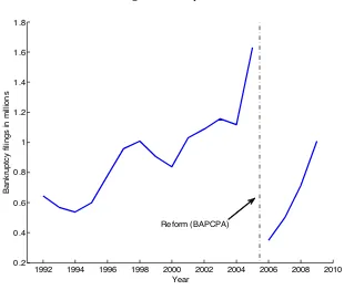
Fig. 1: Bankruptcies

1992 1994 1996 1998 2000 2002 2004 2006 2008 2010

0.2 0.4 0.6 0.8 1 1.2 1.4 1.6 1.8

Year

Bankruptcy filings in millions

Reform (BAPCPA)

model with a similar insurance choice to analyze the effects of tax policy on the medical insurance

market. Attanasio et al. (2008) develop a general equilibrium life-cycle model to study alternative

funding mechanisms for Medicaid. Neither paper discusses unsecured credit, bankruptcies, or health

care reform. To the best of our knowledge, there is no other paper that evaluates the 2010 health care

reform in the general equilibrium framework.

The paper is organized as follows. In Section 2, we present a few facts about bankruptcy and health

insurance reform in the United States. In Section 3 we introduce the model. Calibration and results are

presented in Section 4 and 5, respectively. Section 6 concludes.

2

Background

In this section we provide background information about bankruptcy in the U.S. We describe the U.S.

2.1

Bankruptcy in the U.S.

In the United States a non-business bankruptcy is designed to help people in financial circumstances

beyond their control such as illness or job loss. Distressed debtors have a choice between restructuring

their debt through Chapter 13 bankruptcy or purging the unsecured debt under Chapter 7 bankruptcy,

which accounts for 70 percent of all bankruptcies. Chapter 7 bankruptcy is appealing as it gives an

opportunity for a fresh start by eliminating the unsecured debt. The consequences are a forfeit of

non-collateralized assets above an exception limit and virtual exclusion from credit markets for a period of

10 years, at which point the bankruptcy is removed from credit records.

Regardless of its drawbacks, Chapter 7 bankruptcy is a prevalent phenomenon, which has been

steadily growing over the last two decades (see Figure 1). In the first half of the 1990s there were roughly

600,000 bankruptcy filings each year (0.3 percent bankruptcy rate1_{). The number of bankruptcies}

reached a peak of 1.6 million (0.55 percent) in 2005 before the enactment of the Bankruptcy Abuse

Prevention and Consumer Protection Act (BAPCPA). The act made it more difficult to file for Chapter

7 bankruptcy. Thus the 2005 spike in bankruptcies represents a buildup preceding the change in the

law. Following the fallout from the new law, the number of bankruptcies has been growing, reaching 1

million in 2009.

The main reason for bankruptcy is job loss, which, according to Sullivan et al. (2000), accounted for

67.5 percent of bankruptcies in 1991. In a recent study Himmelstein et al. (2009) conducted the first

survey based on a national random sample of 2300 bankruptcy filers. They found that 62.1 percent of

bankruptcies2_{in 2007 were due to illness or medical bills (see Table 1). Relative to their previous study}

(Himmelstein et al. (2005)), medical bankruptcy increased by 50 percent (in relative terms) between

2001 and 2007. In the same time period, health insurance premiums grew by 78 percent (Claxton et al.

(2007)), and the number of uninsured increased by 1 percent from 18.5 percent to 19.7 percent.3

As pointed out by Livshits et al. (2007), bankruptcy is a form of insurance as it allows individuals

to smooth consumption across states by purging debt in a contingency. It is an especially attractive

1

Bankruptcy rate is defined as the number of bankruptcy filings per capita. 2

The estimates of medical bankruptcy vary widely. Dranove and Millenson (2006) put medical bankruptcy in 2001 at as low as 17 percent, while Himmelstein et al. (2005) estimated it at as high as 54.5 percent. These wide discrepancies in estimates come from the limited data. Studies based on national data sets like the PSID can identify only a small number of bankruptcies (e.g. 74 respondents in the PSID). Usually data sets with bankruptcy questions have limited medical information and vice versa. Thus it is hard to identify income loss due to illness. A majority of studies on medical bankruptcy were based on court records, where medical debt can be disguised as credit card debt or mortgages. These issues were addressed by Himmelstein et al. (2009).

3

Tab. 1: Medical cause of bankruptcy, 2007

Cause of bankruptcy:

% of all bankruptcies

Debtor said medical bills were reason for bankruptcy

29.0

Medical bills >$5000 or >10% of annual family income

34.7

Mortgaged home to pay medical bill

5.7

Medical bill problems (any of above 3)

57.1

Debtor or spouse lost

≥

2 weeks of income

due to illness or became completely disabled

38.2

Debtor or spouse lost

≥

2 weeks of income

to care for ill family member

6.8

Income loss due to illness (either of above 2)

40.3

Debtor said medical problem of self

or spouse was reason for bankruptcy

32.1

Debtor said medical problem of other

family member was reason for bankruptcy

10.8

Any of above

62.1

Source: Table 2 in Himmelstein et al. (2009)

form of insurance against a rare catastrophic event like illness, for example, for young cohorts who are

relatively healthy. But bankruptcy impairs one’s ability to smooth consumption intertemporally due

to exclusion from credit markets and higher interest rates. The latter is a general equilibrium effect as

lenders have to compensate for losses from bad loans. Since lenders price loans to adjust for the risk of

default, people who want to borrow the most have to pay a higher interest rate. This particularly affects

young cohorts, who are at the lowest point of their earnings profile, and therefore rely on borrowing to

smooth their consumption.

One argument in the health care reform debate is that bankruptcy is not the right way to insure

against health shocks. The motivation for the reform was to provide affordable medical coverage to

2.2

Health care system and its reform

In the United States, the health insurance system is divided into public and private sectors. The largest

part of the population, 67 percent in 2007, has private health insurance; 9 percent purchase coverage

directly in the individual market and 59 percent are insured through their employers in the group market.

Public insurance covers 29 percent of the population.4 _{It consists of Medicare, Medicaid, and military}

insurance programs. Medicare insures retirees over 65 and people with certain conditions like ALS and

kidney failure. It covers 14.3 percent of the population. Medicaid is a program covering children, young

mothers, pregnant women, the blind, and the disabled; it is a means-tested program for low-income

individuals only. Medicaid covers 14.1 percent of the population. Military programs primarily insure

veterans and dependents of active-duty military personnel. They cover 3.8 percent of the population.

The remaining 15.4 percent is uninsured.

This fraction of uninsured is the highest among the OECD countries, all of which have universal

health coverage except the United States. The main objective of the 2010 health care reform5 _{is to}

attain close-to-universal coverage in a market-driven health insurance system. Cost containment and

improvement in health care quality are secondary objectives. The reform bill is very complex (it has

over 2000 pages); thus we will outline only the main provisions that we model and the issues they are

designed to address.

Lack of health insurance is prevalent among low-income and middle-class households. The Census

Bureau reports that in 2008 the fractions of people without health insurance in households with income

below $25,000 and with income in the $25,000 - $50,000 bracket was 25.4 and 21.1 percent, respectively.

Uninsured adults with income below the federal poverty level6 _{(FPL) are usually not eligible for}

Medi-caid, which mainly covers children and pregnant women. Those uninsured with income above the FDL

are either unemployed or working for an employer that does not offer group coverage. Many individuals

find non-group insurance unaffordable. In their national survey, the Kaiser Foundation (2010) reports

that an average non-group insurance premium is $3,606 for single coverage with an average deductible

4

Types of coverage are not mutually exclusive; people can be covered by more than one type of health insurance during the year. Source: “Income, Poverty, and Health Insurance Coverage in the United States: 2007,” U.S. Census Bureau.

5

The 2010 health care reform consists of Patient Protection and Affordable Care Act (PPACA), which was signed into law by President Barack Obama on March 23, 2010, and the Health Care and Education Reconciliation Act of 2010 (signed into law on March 30, 2010).

6

of $2,498, and $7,102 for a family plan with an average deductible of $5,149. Given that the median

household income was $50,303 in 2008, the premium in the individual insurance market combined with

the out-of-pocket expenditures takes a significant portion of household income.

The reform facilitates obtaining coverage for low- and median-income households. It expands

Med-icaid to all individuals (including adults without dependent children) under 65 with income up to 133

percent of the FPL. Those enrolled are guaranteed a benchmark benefit package that provides

essen-tial benefits. Individuals and families with income between 133-400 percent of the FPL are eligible to

receive premium credits to purchase health insurance through the Exchange.7 _{Credits are calculated}

so that the insured premium contribution is no more than a specific percentage of income (Table 7).

In order to reduce out-of-pocket expenditures the government will provide cost-sharing subsidies. The

cost-sharing credits reduce co-payments and deductibles so that out-of-pocket expenditures are no more

than a specific percent of total medical spending for a given income level (Table 8).

The high premium of non-group insurance is not the only reason for people to stay uninsured. Many

industry practices are widely criticized for contributing to the inaccessibility of coverage for some people.

The unregulated non-group insurance market allows insurance companies to price discriminate based on

individual characteristics like health. People with preexisting medical conditions have to pay extremely

high premiums if they are not denied coverage outright. The practice of rescinding or denying coverage

renewal due to medical conditions, even though sporadic, has attracted a lot of media attention and

public criticism. All these practices have been prohibited in the group insurance market and now the

reform prohibits them in the non-group insurance market as well.

There is no doubt that these new market restrictions will contribute to increases in the insurance

premium. This will consequently impair insurers’ abilities to pool risk as healthy individuals will decide

to stay uninsured. To alleviate the adverse selection problem common in health insurance markets, and

to maintain a wide enough pool for risk-sharing, the reform imposes a tax penalty for a lack of health

insurance. The penalty is the greater of 2.5 percent of household income or $695 per person up to a

maximum of $2,085 per family. Similarly, employers are penalized for not providing adequate group

insurance coverage. Companies with more than 50 employees have to pay $2000 for each employee who

receives a premium subsidy for individual insurance purchase through the Exchange.

7

We are able to model the most important elements of the reform, described above. We briefly

summarize other details of the reform below. The secondary objective of the reform is to contain the

growing cost of health care. In the last decade, health care expenditures grew from 13.5 percent of GDP

in 1998 to 16.2 percent of GDP in 2008.8 _{A large part of health care expenditures is administrative costs.}

According to Kahn et al. (2005), administrative costs accounted for 25 percent of private health care

spending in 2000 in California; a large portion of it, 20-22 percentage points, was attributed to billing

and insurance-related costs. The reform imposes industry-wide administrative simplification measures.

Insurance companies are required to spend at least 80-85 percent of group and individual plan premiums

on clinical services and quality improvement or to provide rebates to customers for the difference.

To reduce health care costs in the long run, the reform promotes preventive care and wellness. This

policy is primarily designed to target obesity and overweight, the prevalence of which reached 33.8 and

68 percent in 2008, respectively (Flegal et al. (2010)). Obesity is a risk factor for many chronic conditions

like diabetes and heart diseases; thus it contributes to raising health care costs. Finkelstein et al. (2003)

report that the combined medical expenditures accounted for 9.1 percent of total annual U.S. medical

expenditures in 1998 attributable to overweight and obesity; at which point the prevalence of obesity

and overweight was 30.5 and 64.5 percent, respectively. The health care bill provides funding for several

preventive care programs. Government insurance programs are encouraged to cover preventive services

at no additional charge. Employers are permitted to offer employees rewards, in the form of premium

discounts, for participation in wellness programs. Small employers can apply for grants to establish

wellness programs.

3

Model

In this section, we present our model in detail. We describe the economic environment, market

arrange-ments, and the household problem. Lastly, we define the equilibrium of our model.

We use the following notation throughout this paper. Households are heterogeneous in agej, credit

ratingd, health insurance typeiH, and assetsa. Each period, households face idiosyncratic uncertainty

about the labor productivity shockz, health statush, insurance offer indicatoriE, and medical

expendi-ture shockm, all of which are described in later subsections. We denote a random vector of idiosyncratic

8

shocks bys≡(iE, h, m, z). The corresponding transition probability is age dependent and denoted by

Πs

j(s!|s). A household is characterized by a vector(j, s, d, iH, a). A measure over households is denoted

byµ.

3.1

Demographics, preferences, and legal environment

The economy is populated by J overlapping generations of households. Each period households face a

positive probability of dying. We denote the conditional probability of dying at agej+ 1 when being

of agej byψj. Each dying, household is replaced by a newly born household. We assume population

remains constant. The measure of newly born households is normalized to1.

Households value only consumption and supply labor inelastically. Preferences are time-separable

with a constant subjective discount factor β. Instantaneous utility over consumption takes CRRA

functional form u(c) = c1−σ

1−σ. In the case of default or a bad credit history, households incur a

non-pecuniary cost of default,λj,which is age dependent.

3.2

Labor endowment

During working age, households receive a stochastic endowment of efficiency units of labor,nj,h, which

depends on age and health status. The mandatory retirement age isjR_{. We adopt the following process}

for effective labor:

lognj,h= ¯nj,h+zj (1)

where n¯j,h is the age- and health-dependent average log-income and zj is a persistent component

fol-lowing an AR(1) process, zj = ρzzj−1+ηj, ηj ∼ N!0, σ2η

"

. Households’ gross income, y, is a wage

multiplied by efficiency units of labor. The detailed description of a wage can be found in Section 3.5.

3.3

Health and medical insurance

Households are heterogeneous in health status,h, which follows an exogenous Markov processπh

j (h!|h)9.

Health transition probabilities vary with household age.10 _{Each period, a household faces an}

idiosyn-9

An alternative approach is to model health as a form of human capital. Health would enter a utility function. Households would have to invest in health to replenish it as it depreciates each period (see Grossman (1972)). Since our focus is on bankruptcy and health insurance we decided to model health in a simple way as an exogenous process. Endogenizing health remains a subject for further study.

10

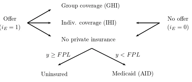
Fig. 2: Insurance choice diagram

Offer

(iE= 1)

Group coverage (GHI)

Indiv. coverage (IHI)

No private insurance

y < F P L

y≥F P L

Uninsured Medicaid (AID)

No offer

(iE= 0)

cratic medical expenditure shock, m, which is randomly drawn from the age- and health-dependent

distributionπm

j,h(m). The medical shock is realized at the beginning of a period and households can

purchase health insurance against this shock one period in advance. There are two competitive health

insurance markets: the individual health insurance (IHI) market and the group health insurance (GHI)

market. All households have access to the IHI market. To purchase group health insurance (GHI), a

household needs to work for an employer who offers a group insurance plan. In the model, households

receive a GHI offer exogenously. The GHI offer flag is denoted byiE. In the data the probability of a

GHI offer is positively correlated with earnings. Thus, we assume thatiE follows an income-dependent

Markov process πE_(i!

E|iE, n). Households have a choice to purchase only one insurance contract or

to stay uninsured.11 _{Low-income households without health insurance are covered by Medicaid. All}

other uninsured households have to pay for all medical expenditures out-of-pocket. Reimbursement for

medical expenses provided by insurance coverage is governed by a transfer functiontrm_{(m, i} H).

In the group insurance market, the law prohibits insurance companies from price-discriminating

based on age or preexisting medical conditions. Thus, the GHI premium pGHI _{is the same for all}

households regardless of their age or health status.12 _{Many employers subsidize group insurance policies}

more general discussion about the relationship between health and income. 11

Some households may be covered by two types of insurance. Unemployed households can purchase a temporary continuation of the group coverage from a former employer under COBRA. To keep the model parsimonious we assume that households can be covered by at most one type of insurance.

12

for their employees as part of a benefit package. In the model a firm pays a fraction ξ ∈[0,1] of the

premium and a household pays the remaining(1−ξ)pGHI_{. A firm will transfer the cost of subsidy onto}

its employees by adjusting wages accordingly (see Section 3.5).

In the individual insurance market, law permits insurance companies to price discriminate based on

age and preexisting medical conditions. Hence, in the model, the IHI premium,pIHI_{(j, h), depends on}

age and health status.

Health insurance markets are perfectly competitive. Insurers cover all losses from contracts with

collected premiums and make zero profits. We assume that insurers do not cross-subsidize the two types

of insurance contracts. In the GHI market, insurers pool the risk over all participants. Thus, the GHI

premium is the discounted average medical expenditure adjusted for a fixed administrative cost,φGHI_.

pGHI = φGHI+

´

trm_{(m, i}

H)1{GHI}(iH)dµ

(1 +r)´

1{GHI}(iH)dµ

(2)

Each IHI contract is priced individually. The IHI premium is the discounted expected payout

ad-justed for a fixed administrative cost,φIHI_.

pIHI(j, h) = φIHI+ψj

´ ´

trm_(m!_{, IHI)π}m

j+1,h"(m!)dm!πhj(h!|h)dh!

(1 +r) (3)

The government runs the Medicaid program, which provides medical coverage to low-income

house-holds. Uninsured working-age households whose income is below the eligibility threshold,yF P L_,

auto-matically qualify for Medicaid coverage. The threshold, yF P L_{, corresponds to the federal poverty level}

(FPL). Medicaid coverage is denoted bytrAID_(m).

All retired households are covered by Medicare. While working, households pay the Medicare tax,

τm, and during retirement pay a premium,pMED. Medicare coverage is governed by a transfer function

trMED_{(m). The program is self-financed.}

We denote out-of-pocket expenditures by χ. Households with private insurance coverage pay m−

trm_{(m, i}

H) out-of-pocket. Copayments for households qualified for Medicaid and Medicare arem−

trAID_{(m) and m−tr}MED_{(m), respectively. Uninsured households with income above the Medicaid}

eligibility threshold, y ≥yF P L_{, are liable for all medical expenditures m. For j ≤ j}R_{, out-of-pocket}

expenditures are defined by

χ=                 

m−trm_{(m, i}

H) ifiH(= 0

m−trAID_{(m) ifi}

H= 0, y < yF P L

m otherwise

(4)

andχ=m−trMED_{(m)for retirees,j > j}R_.

3.4

Credit market

Households can save and borrow. The incentive to borrow comes from life-time consumption smoothing

and precautionary saving motives. The former is due to the hump shape of the life-cycle income

profile. The latter is a consequence of the idiosyncratic productivity and medical expenditure shocks

faced by households. Borrowing is in the form of one-period unsecured loans. We allow households

to file for bankruptcy and discharge their debt. The credit market is perfectly competitive. Creditors

incorporate the likelihood of default into the price of unsecured loans to ensure that they break even

on each loan. In order to forecast a probability of default in the next period, creditors observe all

household characteristics: age,j, and idiosyncratic shocks, s.13 _{So the price of each loan depends on}

those characteristics,(j, s), and the quantity borrowed, a!_{. We denote the loan price byq}

j(s, a!).

Creditors compute the probability of default, πj(s, a!), on a loan of size a! using the household’s

default decision rule,d∗

j,d(s, a!).

πj(s, a!) =

ˆ

d∗

j+1,0(s, a!) Πj(s!|s)ds! (5)

Then, the zero-profit condition implies

13

qj(s, a!) =

  

 

ψj

1+r fora

! _≥0

ψj(1−πj(s,a"))

1+r fora

! _<0

(6)

Notice that we account for a possibility of losses and gains due to the death of some borrowers and

depositors.

3.5

Production

There is a continuum of competitive firms that operate a constant return-to-scale technologyF(K, L).

The marginal products of capital and labor are r and w, respectively. If a firm offers group health

insurance, it pays a fraction, ξ, of the premium for each insured worker. The firm’s cost of health

insurance per efficiency unit of labor is

cGHI =ξpGHI

´

j<jR1{GHI}(iH)dµ

´

j<jRn1{1}(iE)dµ (7)

whereµis a measure of households.

For the zero-profit condition to hold, firms must adjust the market wage rate for their cost of health

insurance. All households that received a GHI offer will receive the adjusted wage,w−cGHI_{, regardless}

of the insurance purchase.

3.6

Medical sector

Health care providers receive a full payment from households that did not file for bankruptcy. But from

defaulted households, providers receive a payment from the insurer,m−χ, and whatever out-of-pocket

expenditures,χ, can be recovered from the household assets,max{0, a}.

Revenue from a household of type(j, d, s, iH, a)is

dj,h(m−χ+max{0, a}) + (1−dj,h)m. (8)

The medical sector clearing constraint is

ˆ

'

d∗j,h(m−χ+max{0, a}) +

! 1−d∗j,h

"

m(

dµ=

ˆ _m

where̟is a sector markup used to clear the medical sector.

3.7

Household problem

When household is working, the timing of events is as follows: (i) all shocks are realized, i.e., labor

productivity z, employer-sponsored insurance offer iE, and medical expenditure shock m, (ii) capital

and labor are employed and households earn wages, and (iii) households make default, consumption,

borrowing/saving, and insurance purchase decisions. An insurance contract is purchased one period

ahead.

The following notation is used for the problem. The value function of a household of age, j, with

a default flag, d, is denoted by Vj,d(s, iH, a). The employer-sponsored insurance offer, health status,

medical shock, and productivity shock are combined to a vectors≡(iE, h, m, z). All expectations below

are taken with respect to the random vectors. The type of health insurance purchased last period and

household net worth are denoted by iH and a, respectively. We refer to the insurance premium by

p(i!

H), which equals (1−ξ)pGHI, pIHI(j, h), or0 depending on the type of coverage purchased. the

out-of-pocket expenditures, χ, the social transfers, trs_{, and taxes, tax, are defined in equations 4, 21,}

and 22.

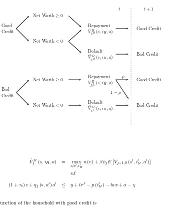
The structure of the value function is illustrated in Figure 3. The household problem is laid out by

cases of credit rating and bankruptcy decision:

1. Let us first consider a household with a good credit history, d= 0. The household can file for

bankruptcy only if its net assets are negative, a−χ < 0. When the household decides to default, it

cannot save or borrow and it has to pay a utility cost of bankruptcy,λj:

ˆ

VjD(s, iH, a) = max c,i"

H

u(c)−λj+βψjE[Vj+1,1(s!, i!H,0)] (10)

s.t

(1 +τc)c ≤ y+trs−p(i!H)−tax (11)

If the household decides to pay its net liabilities or if its net assets are nonnegative, then it faces the

Fig. 3: Household problem diagram

Good Credit

Bad Credit

Net Worth≥0

Net Worth<0

Net Worth≥0

Net Worth<0

Repayment

ˆ

VR

j,0(s, iH, a)

Default

ˆ

VD

j,0(s, iH, a)

Repayment

ˆ

VR

j,1(s, iH, a)

Default

ˆ

VD

j,1(s, iH, a)

t t+ 1

Good Credit

Bad Credit

Good Credit

Bad Credit

ρ

1−ρ

ˆ

VjR(s, iH, a) = max

c,a"_,i" H

u(c) +βψjE[Vj+1,0(s!, i!H, a!)] (12)

s.t

(1 +τc)c+qj(s, a!)a! ≤ y+trs−p(i!H)−tax+a−χ (13)

The value function of the household with good credit is

Vj,0(s, iH, a) = max

) ˆ

VD

j (s, iH, a),VˆjR(s, iH, a)

*

(14)

2. A household with a bad credit history,d= 1, pays a utility cost of bankruptcy,λj, which can be

interpreted as a default stigma. If the household has non-negative net assets,a−χ≥0, it can save and

it will have a good credit rating next period with a positive probability,ρ. Given these conditions, the

Vj,1(s, iH, a) = max c,a"≥0,i"

H

u(c)−λj+βψj

      

ρE[Vj+1,0(s!, i!H, a!)] +

(1−ρ)E[Vj+1,1(s!, i!H, a!)]

(15)

s.t

(1 +τc)c+qj(s, a!)a!≤y+trs−p(i!H)−tax+a−χ (16)

The household with negative net assets, a−χ <0, pays only up to its assets and cannot save or

borrow this period. The household carries a bad credit rating to the next period.14

Vj,1(s, iH, a) = max c,i"

H

u(c)−λj+βψjE[Vj+1,1(s!, i!H,0)] (17)

s.t

(1 +τc)c ≤ y+trs−p(i!H)−tax (18)

Wage is conditional on receiving a GHI offer

y=        !

w−cGHI"

n ifiE = 1

w·n otherwise

(19)

Taxable labor income is defined as

yt=

      

(1−0.5τm)y−0.5τssmin{y,y¯} −p(i!H) ifi!H =GHI

(1−0.5τm)y−0.5τssmin{y,y¯} otherwise

(20)

Notice that half of the Social Security tax paid is deductible. The other half is paid by the employer,

but through wages, the household pays for it in full; thus the entire Social Security tax is effectively

paid by the household. There is no tax base for Medicare. Tax liabilities consist of income taxT(y),

14

Social Security, and Medicare.

tax=T!

yt"

+τssmax{y,y¯}+τmy (21)

Social assistance is a means-tested transfer, which is based on assets and income,15

trs_{= max{0, c−max{0, a} −y} (22)}

3.8

Retirement

When retired, a household receives a pension,ss=υwnjR+ Υw, equal to a fraction of the last working

period’s income plus a fraction of average income in the economy. Recently retired households,j =jR_,

may still have individual or employer-sponsored health insurance. During the first year of retirement,

the household is not covered by Medicare but only by private health insurance if purchased last period.

Households pay the mandatory Medicare premium,pMED_{, one period ahead starting in the first year of}

retirement. Medical expenditures are partially covered by Medicare and partially out-of-pocket. Retired

households do not pay income tax. Bankruptcy is permitted during retirement. After the first period of

retirement, the group insurance offer indicator,iE, is dropped from the state space as it is redundant.

During retirement the budget constraint of a household with good credit that repays its debt is

(1 +τc)c+qj(s, a!)a!≤ss−pMED+trs!ss−pMED, a"+a−χ (23)

A household with bad credit and positive net assets has the same budget constraint with the

ad-ditional no-borrowing restriction, a! _{≥ 0. The budget constraint of a household that purged debt,}

regardless of its credit rating, is

(1 +τc)c≤ss−pMED+trs!ss−pMED, a" (24)

Social assistance during retirement is based on Social Security net of the Medicare premium:

trs= max+

0, c−max{0, a} −!

ss−pMED",

(25)

15

3.9

Equilibrium

A steady-state competitive equilibrium is a set of prices{w∗, r∗}, a non-negative loan price functionq∗,

a default probability functionπ∗

j, a set of health insurance premiums

+

p∗GHI_{, p}∗IHI_(·),

, a non-negative

hospital markup̟, a value functionV, decision rulesc∗_{(·), d}∗_{(·), a}!∗_{(·), and a probability measureµ}∗

such that:

1. Given prices w∗_{, r}∗_{, q}∗_{, p}∗GHI_{, p}∗IHI_{, the value function V and decision rules c}∗_{(·), d}∗_{(·), a}!∗_(·)

solve the household’s optimization problem.

2. Pricesr∗ _andw∗ _{are given by the firm’s marginal productivity of capital and labor:}

r∗ _{= α(K}∗_/N∗₎α−1

−δ (26)

w∗ = (1−α) (K∗/N∗)α (27)

3. A wage at a firm offering GHI is adjusted for the employer’s cost of insurance (eq. 7).

4. The health insurance company is competitive and the insurance premiums satisfy (eq. 3, 2).

5. Loans are priced by financial intermediaries according to a zero-profit condition (eq. 6).

6. The hospital sector clears (eq. 9).

7. The labor market clears,N∗₌´

ndµ∗_.

8. The capital market clears

K∗=

ˆ

q∗a!∗dµ∗+

ˆ

p(i!H)dµ∗ (28)

where the latter term is interest earned by insurance companies on premiums.

9. Social Security and Medicare are self-financed

ss

ˆ

j≥jR

dµ = τss

-j<jR

ˆ

min{y,y¯}dµ (29)

ˆ

j≥jR

trMED(m)dµ∗ = τm

ˆ

j<jR

ydµ∗+pMED

ˆ

j≥jR

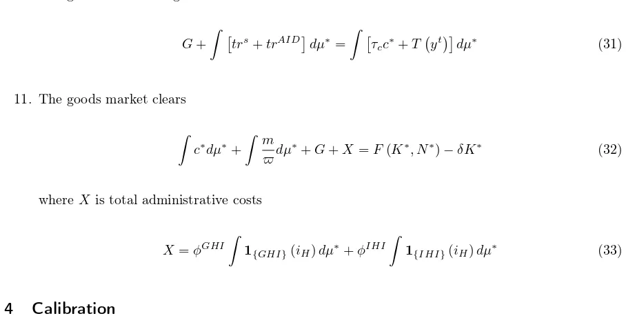
10. The government’s budget is balanced

G+

ˆ

'

trs+trAID(

dµ∗=

ˆ

'

τcc∗+T!yt"(dµ∗ (31)

11. The goods market clears

ˆ

c∗dµ∗+

ˆ _m

̟dµ

∗_+G+X=F(K∗_{, N}∗₎₋

δK∗ (32)

where X is total administrative costs

X =φGHI

ˆ

1{GHI}(iH)dµ∗+φIHI

ˆ

1{IHI}(iH)dµ∗ (33)

4

Calibration

In this section we specify the parameters of the model. Since we do not model the bankruptcy reform

of 2005, we calibrate the model to 2004. All calibration details are presented in Appendix A. Table

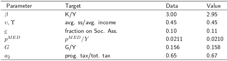
2 summarizes key parameters. Calibrated parameters with corresponding target statistics are listed in

Table 3.

4.1

Model Specification

Demographics and Preferences: Households enter the model economy at age 20 and retire at age 65

(JR _{= 46). The survival probabilitiesψ}

j are taken from Bell and Miller (2002). All households live for

no longer than 80 years (J= 60). The utility function is CRRA with a relative risk-aversion coefficient

σ= 2.0, which implies an intertemporal elasticity of substitution of 0.5, in the middle of the range of

micro estimates in the literature (see Attanasio (1999), for a survey). In the U.S., bankruptcy stays on

a credit history for 10 years. We set the probability of restoring a good credit rating, ρ, to 0.1, which

gives an average duration of exclusion from access to credit of 10 years. The discount rate,β = 0.983,

is calibrated to equate the capital-output ratio to 3.0.

We assume that our non-pecuniary cost of default,λj, monotonically decreases with age. As pointed

out by Fay et al. (2002), bankruptcy carries a stigma, which affects job prospects and consequently

over the remaining lifetime. We assumeλj takes the functional formmax(aλ−bλ·j, cλ). Parameters

{aλ, bλ, cλ}are calibrated to match the bankruptcy profile from the Survey of Consumer Finances taking

values{3.5,0.1,0.05}. We assume that all households are born with zero assets and good credit ratings.

Technology: The aggregate production function is Cobb-Douglas in capital and effective labor:

Y =ZKα_L1−α ₍₃₄₎

We set the capital share of output,α, to0.36, and the physical depreciation rate,γ, to8percent. Total

factor productivity,Z, is chosen so that income per household ($42,414 in 2004) is normalized to1.0in

the steady state.

Earning process: An income age-profile is estimated from the Medical Expenditure Panel Survey

(MEPS) using methodology from Hubbard et al. (1994). For the estimation details, see Appendix A.2.

The stochastic process for the idiosyncratic part of log-wages is an AR(1) process with persistence

pa-rameterρzand unconditional standard deviationσ2z. We setρzto0.99, which is in line with Storesletten

et al. (2004), and we calibrateσz2to 0.29 to match the earnings Gini, which is 0.63 in the U.S. (Castaneda

et al. (2003)). Both values are in line with the estimates from Storesletten et al. (2004). The process is

discretized using the Tauchen and Hussey (1991) method with 9 grid points.

Health and medical expenditure process: We define household health status,h, as a binary variable

taking values: good (1) or bad (0). The age-dependent Markov transition matrix for health status is

estimated from MEPS using a logistic regression model (see Appendix A.3). For the medical expenditure

shock, we use a four-point grid. The distribution over the grid points is fixed. To capture a fat tail

distribution of medical events, we choose the probabilities for the grid points to be{0.5,0.4,0.09,0.01}.

The persistence of medical expenditures comes from the persistence of the health shock. The shock

values depend on age and health. Figure 12 shows the shock values. The estimation details can be

found in Appendix A.4.

Health insurance: In the data, households with high income are more likely to work for a company

offer. Thus, we assume the GHI offer indicator,iE, to follow a Markov process conditional on household

income,πE_(i!

E|iE, n). The initial measure of households with a GHI offer is35.7percent. More details

on the estimation can by found in Appendix A.5.

We obtain the medical insurance transfer function,trm_{(m, i}

H), by estimating the coverage rate,q=

trm_{/m. In MEPS, the private insurance coverage rate increases with the size of medical expenditures.}

Therefore we choose a cubic polynomial as a functional form for the coverage rate. For Medicaid and

Medicare, we fix q at a value corresponding to the mean coverage rate. The estimation details are in

Appendix A.6.

In the National Health Expenditure Accounts, the net cost of private health insurance in 2004 is $85.8

billion. In the same year 201 million people had private health coverage. Thus, the fixed administrative

cost is $427 per person or $1,067.5 per average household with 2.5 people. We set bothφGHI _andφIHI

to the latter value. According to MEPS in 2004, an average employer-sponsored insurance premium is

$3,705and an average employee’s contribution is $671. Thus, we set the employer’s share of the GHI

premium,ξ, to82percent.

Government: Government consumption, G, represents federal, state, and local government

con-sumption expenditures excluding social benefit payments, interest payments, and subsidies. It is

cali-brated to match its share of GDP, which is15.7percent in 2004 (U.S. Government 2009).

Our income tax is composed of progressive and proportionate taxes. The latter represents all taxes

other than income and consumption tax. The former takes a functional form borrowed from Gouveia

and Strauss (1994).

T(y) =a0

)

y−!

y−a1_+a

2"

−1/a1*

+τyy (35)

Parametera0is the maximum marginal tax rate,a1governs the curvature of the progressive tax, and

a2 is a scaling parameter. We take their values,a0= 0.258,a1= 0.768, from the estimates by Gouveia

and Strauss (1994) to preserve the shape of the progressivity of the U.S. tax system. The parametera2

is calibrated to match the portion of the progressive part of income tax in the total income tax collected.

This target is set to63percent, which is the 10-year average fraction of the individual income tax to the

total Internal Revenue collections.16 _{Parameter τ}

y is used to clear the government budget constraint

(31). A consumption tax rate,τc, is set to5.6percent following Mendoza et al. (1994).

16

A minimum consumption floor,c, is calibrated to match the fraction of households on social welfare,

which the CPS reports at10.2percent in 2004. We set the Medicaid eligibility threshold to the federal

poverty level,yF P L_{, which is calibrated to match the fraction of people covered by Medicaid.}

Social Security and Medicare: A household retires at the mandatory retirement age, jR _{= 65. We}

set the Social Security benefit parameters,υ andΥ, to0.4 and 0.2, respectively, to match an average

replacement rate of45percent following Whitehouse (2003). The Social Security tax,τss, is determined

so that Social Security is self-financed. In the benchmark economy we get the equilibriumτss= 11.49,

which is approximately the tax rate of Social Security’s Old-Age, Survivors, and Disability Insurance

(OASDI) program of12.4percent in 2004.

In 2004 the Medicare Part B premium was $799.20 annually, or about 2.11 percent of GDP per

capita. We set the Medicare premium,pMED_{, to match this ratio. The Medicare tax rate,τ}

m, is pinned

down by the budget clearing of Medicare, which is self-financed. Since the Medicare coverage rate,

trMED_{(m)/m, is scattered without any visible pattern, we set it to0.48, which is the average Medicare}

coverage rate in MEPS.

5

Results

In this section we elaborate on results from the benchmark model. We describe how each element of

the reform is modeled. The impact of the reform on insurance markets and bankruptcy is presented.

Lastly, we evaluate the welfare implications and decompose the redistribution and insurance market

restructuring components of the reform.

5.1

Benchmark model

Even though we did not target bankruptcy and health insurance statistics directly, our model succeeds

in matching them not only qualitatively but quantitatively as well. The life-cycle dimension of these

statistics is also replicated reasonably well.

The overall bankruptcy rate is 1.0 percent (0.98 percent in the data). In the model we define medical

bankruptcy as the fraction of filers who would not have defaulted had they not received a bad medical

Tab. 2: Benchmark parameters

Parameter

Description

Values

Target/Source

Preferences

β

discount factor

0.983

K/Y=3.0

σ

risk aversion

2.0

ρ

prob. of good credit

0.1

10 years exclusion

{a

, b

, c

}

cost of bankruptcy

{

3

.

5

,

0

.

1

,

0

.

05

}

bankruptcy profile

Technology

α

capital share

0.36

γ

depreciation rate

0.08

Labor

ρ

persist. coeff.

0.99

Storesletten et al. (2004)

σ

std. dev.

z

0.29

earnings Gini=0.63

Other

ξ

firm premium share

0.89

MEPS, 2004

φ

,

φ

fixed admin. cost

$1,067.5

NHEA

Government

a

, a

prog. income tax

0

.

258

,

0

.

768

Gouveia and Strauss (1994)

a

prog. income tax

2

.

16

P rog./T tax

= 0

.

65

τ

prop. income tax

0

.

013

const. clearing

τ

consumption tax

0

.

06

Mendoza et al. (1994)

τ

Social Security tax

0

.

1

const. clearing

τ

Medicare tax

0

.

012

const. clearing

G

gov. consumption

18

.

92

G/Y

= 0

.

16

Tab. 3: Calibrated parameters

Parameter Target Data Value

β K/Y 3.00 2.95

υ,Υ avg. ss/avg. income 0.45 0.45

c fraction on Soc. Ass. 0.10 0.11

pMED _pMED_{/Y 0.0211 0.0210}

G G/Y 0.156 0.158

a2 prog. tax/tot. tax 0.65 0.67

Tab. 4: Benchmark: bankruptcy

Medical Medical bk. Med. bk. w/o

% Bankruptcy bankruptcy share health ins.

Data 0.98 0.61 62.1 31

Model 1.01 0.76 75.97 30

of all bankruptcies (62.1 percent in the data). Among medical bankruptcy filers 30 percent had no

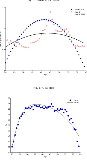
health insurance (31 percent in the data). In Figure 4 we plot a fitted-value profile of bankruptcy from

the model and from the 2004 Survey of Consumer Finances. With respect to the life-cycle literature on

bankruptcy the model achieves a good fit of the bankruptcy profile. Only early in life does the model

generate more bankruptcies than in the data. A possible reason for this discrepancy is a lack of parental

transfers, which allow young households to cushion negative income and medical expenditure shocks.

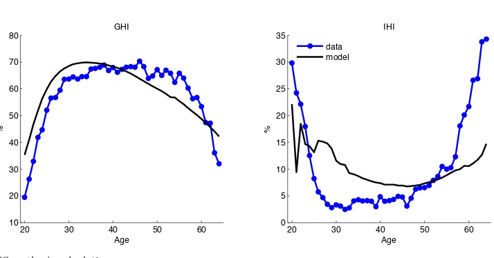
Figure 5 presents the offer and acceptance rate profiles. The group insurance offer rate is 67.0 percent,

which is a little higher than in the data (65.3 percent). Among households that received an offer, 89.2

percent accepted it (91.2 percent in the data). The profile of the acceptance rate is endogenously

generated and matches the data quite well (Figure 6).

Tab. 5: Benchmark: insurance

Group Insurance Insurance Coverage

% offered accepted GHI IHI Medicaid Uninsured

Data 65.31 91.22 59.58 9.76 10.81 19.85

Model 67.02 89.16 59.78 10.26 10.13 19.83

Fig. 4: Bankruptcy profile

20 25 30 35 40 45 50 55 60 65

0 0.5 1 1.5

Age

Bankruptcy rate, %

data, fitted model model, fitted

Fig. 5: GHI offer

20 25 30 35 40 45 50 55 60 65 30

35 40 45 50 55 60 65 70 75 80

Age

%

Fig. 6: Insurance take-up rates

20 30 40 50 60

10 20 30 40 50 60 70 80

GHI

Age

%

20 30 40 50 60

0 5 10 15 20 25 30 35

IHI

Age

%

data model

Source: MEPS, author’s calculations.

The results on insurance coverage are presented in Table 5. Less than a quarter of households are

uninsured (19.7 percent in the model and 19.9 percent in the data). Medicaid covers 10.1 percent of

households (10.8 percent in the data). Group and individual insurance coverage is 59.8 and 10.3 percent,

respectively (59.6 percent and 9.8 percent in the data). Medicaid coverage is targeted in calibrating the

federal poverty level,yF P L_{, but the share of uninsured and the profile of those with private coverage}

are endogenously generated by the model (Figure 6) and match the data well. We consider the model’s

ability to replicate health insurance statistics a success.

The premiums and risk pools are reported in Table 6. In MEPS, the fraction of households in bad

health is 14.7 percent in both private insurance markets and 18.4 percent among the uninsured. The

model replicates the GHI risk pool quite well at 14 percent. In the IHI market, the model generates a

worse pool than in the data. One possible explanation is that insurance companies can improve their

pool by not accepting sick individuals or canceling an existing policy, but we do not model the denial

and rescission of coverage.

5.2

Policy experiments

In our experiments we keep the government consumption, G, consumption tax, τc, and progressive

income tax,(a0, a1, a2)unchanged from the benchmark. The proportionate part of income tax adjusts

Tab. 6: Benchmark: premium and risk pools

Data Model

Individual Family

GHI $3,383.00 $9,068.00 $3,296.79 IHI $1,786.00 $3,331.00 $1,292.33

Bad Health, % Data Model GHI 14.7 15.50

IHI 14.7 20.91 Uninsured 18.4 13.98

Source: Kaiser FamilyFoundation 2004 (premium); MEPS (health).

We keep Social Security benefits, ss, and the Medicare premium,pMED_{, at the benchmark level. The}

tax rates,τs andτm, adjust to balance both systems.

We can evaluate the welfare effects of policies only by comparing two steady states, before and after

the reform, through the consumption equivalent variation (CEV). The consumption equivalent variation

measures the percentage increase in the household’s initial consumption required to make the household

indifferent between benchmark and reform steady states. Given the form of the utility function, the

welfare measure is given by

CEV =

.´

VR

j,ddµ∗j=0,d=0

´

VB

j,ddµ∗j=0,d=0

/1/(1−σ)

−1 (36)

where VB _{and V}R _{are the indirect utility functions at birth of households with a good credit rating}

associated with the benchmark and the reform, respectively.

5.2.1 Health reform components

The health care reform bill is very complex, but the core of the reform can be summarized by five

essential provisions. In this section we describe how each element of the health reform is modeled.

1. Individual mandate

The reform requires all individuals to maintain minimum essential coverage. Those without

cov-erage pay a tax penalty of 2.5 percent of income with a minimum of $95 in 2014, $325 in 2015,

and $695 in 2016. In our experiment we take the latter as a minimum penalty.

2. Prohibition of discrimination based on health

char-acteristics, including health. The common practice was to deny new coverage due to preexisting

conditions or refusing to renew coverage due to health problems. The reform requires insurers

to accept every individual who applies for coverage and to renew coverage regardless of health

status, utilization of health services, or any other related factor. It prohibits denying coverage due

to any preexisting condition or discrimination against those who have been sick in the past. We

model this provision by allowing the individual premium to vary with age only. Not knowing the

health status of an applicant, an insurer has to use the distribution of health over age to calculate

expected expenditures. The new IHI premium is given as

pIHI(j) =φIHI+ψj

´

trm_(m!_{, IHI)dµ(·|j+ 1, i}!

H=IHI)

(1 +r) (37)

3. Expanding Medicaid to all in poverty

Prior to the reform Medicaid covered only children, pregnant women, and people with disabilities

from families with income below the FPL. Many people and family members were not covered,

i.e., all adult males and females without children. To provide coverage to all people in poverty, the

reform extends Medicaid coverage to all individuals in families with incomes less than 133 percent

of the FPL.

In the benchmark model, the Medicaid coverage rate was estimated using all households under 100

percent of the FPL whether eligible or not. In MEPS, Medicaid covered only 37.38 percent of all

medical expenditures on average, even though it covered 71.02 percent of medical expenditures for

eligible individuals. To account for the expansion of coverage to everyone in poverty, we increase

the Medicaid coverage rate for households to the pre-reform level for eligible individuals only,

trAID_{(m)/m= 0.71.}

4. Premium subsidies

The reform provides premium subsidies for individuals and families with income between 133

percent and 400 percent of the FPL. Households are not eligible for the credit if they are covered

by Medicaid or if their employer offers group insurance coverage. The subsidy depends on income,

and its amount is determined so that the premium would not exceed a percentage of income as

Tab. 7: Premium subsidies

Income Level Maximum Premium % of FPL % of Income

Up to 133 2

133-150 3-4

150-200 4-6.3

200-250 6.3-8.05 250-300 8.05-9.5

300-400 9.5

Note: The amount of premium credits is determined so that the individual/family premium contribution is limited to the percent

of income listed above.

Tab. 8: Cost-sharing reduction

Income Level Out-of-pocket spending limits % of FPL as a fraction of the HSA limit

100-200 1/3

200-300 1/2

300-400 2/3

advance. They are fully funded by the government from general taxation. We implement the

subsidies as an instantaneous adjustment to the premium.

5. Cost-sharing reduction

The reform enacts limits on out-of-pocket expenditures for those with income below 400 percent

of the FPL. This cost-sharing reduction applies to non-group policies only. The reference point is

the standard out-of-pocket spending limits for Health Savings Accounts (HSA), which are $5,950

for individuals and $11,900 for families in 2010. The out-of-pocket maximum limits are set at

one-third of the HSA limit for those between 100-200 percent of the FPL, one-half of the HSA

limit for those between 200-300 percent of the FPL, and two-thirds of the HSA limit for those

between 300-400 percent of the FPL (Table 8). In our analysis we take the HSA limit to be equal

to $11,900. We implement cost-sharing subsidies by imposing out-of-pocket limits on the payouts

of IHI coverage. The higher premium is reimbursed by the premium subsidies only if households

Fig. 7: Insurance take-up rate, reform

/home/mkuklik/Documents/Research/default-health/draft/h28/ins_reform.eps

5.2.2 Reform implications

Health Insurance Market

Table 9 presents the impact of the reform on insurance markets. The reform achieves its goal of almost

universal coverage. The number of uninsured drops to 4.1 from 19.8 percent. This is in line with the

Congressional Budget Office’s 5 percent estimate of the post-reform uninsured rate.17 _{Medicaid absorbs}

5.5 percentage points of the uninsured as the eligibility income threshold goes up to 133 percent of the

FPL. Private-sector coverage draws the remaining 10.1 percent of the uninsured. The group insurance

take-up rate increases by 3.6 percent, to 63.3 percent. The individual mandate is mainly behind the

increase in group insurance market share. Without the penalty in the reform the GHI take-up rate

would fall to 60.1 percent. The non-group insurance market participation rate increases by 6.7 percent,

to 16.9 percent. The result is driven by the combination of premium subsidies, which make coverage

more affordable, and the individual mandate, which increases the cost of being uninsured. When either

component is removed from the reform, the IHI take-up rate drops below the benchmark level.

The prohibition of discrimination creates a new risk-sharing mechanism. Inability to price coverage

based on health forces insurers to increase premiums as they spread the risk related to a lack of

informa-tion about health over all insured households within each age group. Intrinsically, healthy households

17

Tab. 9: Reform with marginal contributions: health insurance

∆from Reform without:

(%) Benchmark Reform Pen

a lt y IH I b y a g e M ed ic a id S u b si d y Co st -s h a ri n g m a rk et re st ru ct u ri n g re d is tr ib u ti o n Insurance

GHI 59.8 63.3 -3.19 0.04 2.07 -0.13 -0.01 65.8 60.3

IHI 10.3 16.9 -7.7 0.57 9.07 -8.79 -0.69 10.2 13.5

Medicaid 10.1 15.6 0.65 -0.06 -10.28 1.97 0.29 10.5 16.2

Uninsured 19.8 4.1 10.24 -0.55 -0.86 6.95 0.4 13.5 10.0

accepted | GHI offered 59.8 63.3 -3.2 0.0 2.1 -0.1 0.0 65.8 60.3

Premium, $

GHI $3,297 $3,389 -$40 $0 -$37 -$1 -$0 $3,356 $3,351

Average IHI: $1,292 $2,816 $119 -$221 -$16 -$167 -$81 $2,511 $2,498

in bad health $1,605 $3,409 -$17 $1,353 -$117 -$65 -$73 $3,252 $4,654

in good health $1,210 $2,652 $11 -$626 $22 -$257 -$67 $2,258 $1,793

% with bad health

GHI 15.5 15.5 0.14 0.01 -0.18 -0.05 -0.01 15.3 15.7

IHI 20.9 21.6 15.63 -0.80 -1.18 5.05 -1.73 25.5 24.7

AID 36.2 25.9 0.09 -0.09 15.66 3.02 1.76 37.1 25.9

Fig. 8: Medicaid and uninsured, reform

/home/mkuklik/Documents/Research/default-health/draft/h28/aidno_reform.eps

subsidize coverage for households in bad health. This drives the healthy individuals out of the non-group

market, putting additional upward pressure on premiums. If the health discrimination provision had not

been part of the reform, the risk pool in the non-group market would have consisted of fewer households

in bad health (20.8 vs. 21.6 percent) and the average IHI premium would have been lower ($2,595 vs.

$2,815). This effect is relatively small due to the presence of the premium subsidies in the counterfactual

experiment. Without subsidies, the prohibition of discrimination would have a much more significant

impact on the non-group insurance market. Subsidies target the healthy households, who would not

buy expensive coverage otherwise. These households are important for hedging risk within the

insur-ers’ risk pools. Without subsidies, the IHI risk pools deteriorate as the fraction of households in bad

health increases by 5.1 percent, to 26.7 percent. Thus, subsidies are crucial to the success of the new

risk-sharing mechanism created by the introduction of the prohibition of discrimination.

Bankruptcy

The reform reduces the bankruptcy rate by a modest 0.06 percentage point (from 1.0 percent to 0.94

percent). The bankruptcy breakdown by the FPL income groups in Table 10 reveals that the bankruptcy

rate drops mainly among households with income below 200 percent of the FPL. The expansion of

Medicaid is responsible for fewer bankruptcies of households below 133 percent of the FPL. Eliminating

Tab. 10: Reform with marginal contributions: bankruptcy

∆from Reform without:

(%) Benchmark Reform Pen

a lt y IH I b y a g e M ed ic a id S u b si d y Co st -s h a ri n g m a rk et re st ru ct u ri n g re d is tr ib u ti o n

Bankruptcy: 1.0 0.94 0 -0.01 0.01 0.03 0.01 1.03 0.94 GHI 8.6 7.4 -1.8 0.0 5.3 -0.8 -0.1 10.3 5.6

IHI 2.4 9.6 -5.0 0.2 33.8 -9.1 0.5 1.7 4.6 Medicaid 48.4 67.3 -0.3 0.9 -33.6 -5.9 -0.9 46.1 68.5 Uninsured 40.6 15.6 7.1 -1.0 -5.5 15.7 0.5 41.9 21.3

Bankruptcy rate (%) by the FPL income group

4.0·F P L≤y 0 0.01 0 0 0 0 0 0.01 0

3.5≤y <4.0·F P L 0.04 0.03 0.01 -0.01 0 0.01 0 0.04 0.03

3.0≤y <3.5·F P L 0.11 0.1 0.06 -0.03 -0.02 0.08 0.01 0.13 0.12

2.5≤y <3.0·F P L 0.16 0.14 0.07 -0.02 -0.01 0.09 0.01 0.17 0.16

2.0≤y <2.5·F P L 0.42 0.49 0.13 0 -0.23 0.3 0.01 0.48 0.59

1.5≤y <2.0·F P L 0.75 0.7 0.1 -0.02 -0.34 0.52 0.06 0.83 0.78

1.33≤y <1.5·F P L 1.48 1 0.12 -0.05 -0.32 1 0.2 1.6 1.05

1.0≤y <1.33·F P L 2.57 1.64 -0.05 -0.01 0.02 -0.08 0.06 2.79 1.59

y <1.0·F P L 2.93 2.66 -0.07 0 0.45 -0.24 -0.05 2.86 2.61

Note: FPL is the federal poverty level, which is the poverty thresholds used for administrative purposes — for instance, determining financial eligibility for certain federal programs.

point among the two lowest FPL income groups. The cost-sharing and premium subsidies contribute

to lowering the bankruptcy rate among households with incomes between 133 and 400 percent of the

FPL. Both policies work progressively by lowering bankruptcies more in the lower income brackets.

In the absence of the cost-sharing provision, the bankruptcy rate in the 130-150 percent and 150-200

percent FPL income groups would increase by 0.2 and 0.06 percentage point. The premium subsidies

have a large impact on the bankruptcy rate. If the reform did not include the premium subsidies, the

bankruptcy rate would rise by 1.0 and 0.52 percentage point with respect to the same FPL income

groups.

groups above 133 percent of the FPL. However, its mechanism differs from the two former provisions.

The penalty for a lack of coverage enhances risk pooling as it induces the low-risk healthy households

to buy coverage. This is distinctly apparent in the IHI market, where the fraction of households in

bad health would increase by 15.63 percent in the reform without the individual mandate. Better risk

pooling leads to lower premiums ($2,816 vs $2,935 without the penalty) and thus higher demand for

coverage. The bankruptcy rate drops as more households purchase health coverage. Notice that the

price effect of enhanced pooling is absent in the GHI market as the pool composition would change

insignificantly without the mandate (by 0.14 percent from 15.5 percent). Group insurance has the tax

incentive mechanism, which has already attracted most households with a group offer to buy coverage

(GHI has89.16 percent acceptance rate). The IHI discrimination provision is the only element of the

reform that increases the bankruptcy rate across all income groups. The higher premium makes coverage

less affordable and thus draws some households into being uninsured. But the effect is very small; a

change in the bankruptcy rate is measured in hundredths of a percentage point.

Overall, medical bankruptcy decreases slightly by 0.06 percentage point (Table 11). The main

contributor to the drop in medical bankruptcies is the premium subsidy, which expands private coverage

to the uninsured. In the counterfactual experiment, it lowers the medical bankruptcy rate by 0.06

percent. By the same token the cost-sharing provision reduces medical bankruptcy by 0.01 percent.

Medicaid expansion affects medical bankruptcy in two opposite ways. On the one hand, it decreases

the number of medical bankruptcies among low-income households below 100 percent of the FPL as

it enhances coverage quality. On the other hand, it increases the number of medical bankruptcies in

all other income groups. In the latter case the Medicaid expansion drives households away from the

private insurance markets, where risk pooling deteriorates and premiums increase. In the absence of

Medicaid expansion, participation in the group and individual insurance markets would increase by 2

and 9 percent, the risk pools would improve by 0.18 and 1.18 percent, and average premiums would

drop by $37 and $16. Fewer households would be uninsured and the fraction of medical bankruptcies

in where health insurance was not purchased would drop by 6.7 percent. Thus, medical bankruptcy

would rise by 0.23 percent among households below 100 percent of the FPL and drop in all other income

groups. The net effect on the medical bankruptcies is -0.05 percentage point. Overall, the Medicaid

expansion causes more medical bankruptcies than it prevents. In a similar fashion, the prohibition