How to cite this paper: Papageorgiou, C.D. (2016) Enclosed Solar Chimney Power Plants with Thermal Storage. Open Access Library Journal, 3: e2666. http://dx.doi.org/10.4236/oalib.1102666
Enclosed Solar Chimney Power Plants
with Thermal Storage
Christos D. Papageorgiou
Electrical Engineering Department, National Technical University of Athens, Athens, Greece
Received 19 April 2016; accepted 23 May 2016; published 27 May 2016
Copyright © 2016 by author and OALib.
This work is licensed under the Creative Commons Attribution International License (CC BY).
http://creativecommons.org/licenses/by/4.0/
Abstract
The main problem associated with intermittent operation of the wind and PV power plants is the lack of low cost electrical storage methods. In the present paper a new type of solar chimney technology that we shall heretofore call “Enclosed Solar Chimney Power Plant technology (ESCP technology) stands for an effective alternative of combining both low cost electricity generation as well as smooth, uninterrupted operation for 24 hours/day and for all 365 days/year. The ESCP technology also has the following benefits in relation to PV technologies: 1) Local manufacturing and use of common material for their construction (steel, glass, concrete and conventional axial fans as air turbines); 2) Easy and low cost maintenance; 3) Longer operating life up to 50 years (its solar chimney up to 100 years); 4) No water consumption; 5) Zero effect on living nature and am-bient; 6) Their empty protected surface area beneath the glassed roofs of their greenhouses can be used for desalination with parabolic trough mirrors.
Keywords
Solar Chimney, Enclosed Greenhouse
Subject Areas: Electric Engineering
1. Introduction
One of the major problems in the wide application of both solar and wind energy power plants is their intermit-tent operation. Although their levelized cost per kWh has already become comparable to the cost of kWh gener-ated by fossil fuels (coal, gas, nuclear), the projected participation up to the year 2035 in overall energy demand is unsatisfactory. The main problem associated with intermittent operation is the lack of sufficiently mature electrical storage methods. According to a recent article by Bill Gates titled “We Need an Energy Miracle”
le-OALibJ | DOI:10.4236/oalib.1102666 2 May 2016 | Volume 3 | e2666 velized KWh electricity generation cost, which do not exceed 10 cents.
In the present paper we intend to show that a new type of solar chimney technology that we shall heretofore call “Enclosed Solar Chimney Power Plant” (ESCP) technology stands for an effective alternative capablity of combining both low generation cost as well as smooth, uninterrupted operation for 24 hours/day and for all 365 days/year. This is achieved with the introduction of a low cost artificial water storage facility which can always be constructed on ground near the base of the solar chimney structure and protected by external winds.
2. The Solar Chimney Power Plant as an Artificial Wind Generator
Conventional solar chimney power plants (Solar Updraft Power Plants) are made of the following cooperative systems:
• The solar air up-drafting system that is made of two parts:
A circular solar collector, which is a circular greenhouse with a transparent roof, that is open to its perimeter. The solar irradiation through the transparent roof of the greenhouse warms the ground beneath the greenhouse, while its transparent roof blocks the thermal radiation of the ground and decreases the thermal losses due to the air convection. Thus the air temperature inside the greenhouse is increasing and this warm air becomes lighter than the ambient air.
Additionally, a cylindrical solar chimney is placed in the center of the circular solar collector, through which the warm air is forced due to its buoyancy to escape towards the upper atmosphere. The escaping warm air is con-stantly replaced by fresh air entering through the open periphery of the greenhouse. So the warm air stream moves constantly, so long as the greenhouse ground gets warmer than the ambient air and this phenomenon can go on for several hours after the sunset.
• The electricity generating power system is made of:
One or more air turbines placed inside the solar chimney (of vertical axis) or around the base of the solar chimney (of horizontal axis), which are forced to rotate by the moving stream of warm air escaping through the solar chimney. The air turbines are engaged, via appropriate gear boxes, to electric generators which are also forced to rotate, generating electricity.
Extensive description and important information about solar chimney technology is posted on the website
https://en.wikipedia.org/wiki/Solar_updraft_tower.
As a result we can say that the solar chimney power plants practically are systems creating artificial wind. The stream of artificial wind entering through the open periphery of their greenhouses and escaping through their solar chimneys, is forcing the air turbines and their engaged electric generators to rotate, generating electricity.
An indicative figure of a conventional solar chimney power plant with one turbine inside the solar chimney is shown in Figure 1.
3. The Enclosed Solar Chimney Power Plant (ESCP)
The enclosed solar chimney power plant (ESCP) is a simpler and lower cost solar chimney power plant, where the name “enclosed” stems from its solar collector (greenhouse) being encircled by a peripheral wall. The air turbines of the ESCPs, without gear boxes, are placed in proper openings on the peripheral wall that is enclosing the solar collector (greenhouse). An indicative model of an enclosed solar chimney power plant (ESCP) is shown in Figure 2(a) &Figure 2(b).
The overall cross section area of the air turbines is several times smaller than the solar chimney cross section area. Thus the air speed entering into the air turbines is also several higher than the speed of the up-drafting warm air inside the solar chimney. Thus the rotational speed of the air turbines is increasing consequently.
A careful choice of the air turbine diameters in relation to solar chimney diameter for optimum efficiency can define their rotational speed to be equal to the generators rotational speed (that depends upon the grid frequency and the number of their pole pairs).
Thus the gear boxes can be omitted and the ESCPs electricity generation system has a lower cost. Further-more ordinary axial air fans, existing in abundance in the market, can be used as reciprocal machines i.e. as air turbines with ESCPs. The existing axial air fans have been tested for many years in many applications and their efficiencies are not less than 70%.
OALibJ | DOI:10.4236/oalib.1102666 3 May 2016 | Volume 3 | e2666
AIR IN
H
Dc Solar Horizontal irradiation
G
AIR IN
AIR OUT
03 03te
d
T
02 T
01 P4
T T T4
[image:3.595.145.485.88.343.2]INLET VANES TURBINE
Figure 1. A schematic representation of a conventional solar chimney power plant of one air
tur-bine placed inside its solar chimney.
(a) (b)
Figure 2. (a) An ESCP made of a octagonal greenhouse enclosed by a peripheral wall and sixteen air turbines placed in proper openings on its peripheral wall. (b) A detail of the previous ESCP greenhouse with one air turbine and its opening’s
air stop.
the turbines air speeds. Thus in order to match continuously the turbine air speed to chimney air speed for an op-timal operation and maximum efficiency and electricity generation we should control the electro-mechanical air stop systems.
The openings, where the air turbines are placed, are equipped with electro-mechanical air stop systems. Every air stop system can be activated separately, in order to close firmly or open the respective opening and release or stop the incoming air stream that is forcing the respective air turbine to rotate.
[image:3.595.88.533.376.538.2]OALibJ | DOI:10.4236/oalib.1102666 4 May 2016 | Volume 3 | e2666 operation of their respective air turbines. Finally the overall electrical power of the ESCP can be increased in a controllable way.
Increasing the operational speed of the air turbines of the ESCPs in comparison to the air speeds forcing the air turbines of a respective conventional solar chimney power plant, can multiply the annual electricity genera-tion several times as will be shown in the next paragraph.
The ground area of the closed solar collector (greenhouse), beneath its glass roof, should be covered with a thin black plastic or elastic carpet, in order to increase the solar irradiation absorbance of the solar collector. Beneath this carpet, in a part near the center, a concrete structure filled with water can be built, in order to in-crease the thermal storage capacity of the ESCP. Thus the ESCP can have a smooth and continuous operation 24 h/day 365 days/year.
The wall at the perimeter of the ESCP protects the thermal storage facility by heavy thermal losses due to ex-ternal winds, especially at night, increasing its electricity generation. Thus ESCP is a solar technology with smooth and non intermittent operation that can be used in proper cooperation with the rest of renewable tech-nologies in order to achieve timely the extinction of fossil fuels from electricity generation.
Thus the main benefits of ESCPs in comparison to standard conventional solar chimney power plants can be summarized as follows:
- Avoidance of gear boxes;
- Use of existing off-the-shelve air turbines (used as axial air fans for instance); - Ability to optimize ESCP’s power output via microprocessor controlled air openings;
- Possibility of enhancing power output via openings of overall smaller cross section area in comparison to chimney cross-section area;
- Wind protected thermal storage facility inside their enclosed greenhouse.
4. Operational Equations for the ESCP
Let us define the overall opening cross section area of the operating air turbines of the ESCP to be AT while the chimney cross section area is ACh=πd2 4 where d is chimney internal diameter. If the air speed passing through the ducted air turbines is UT and the chimney air speed is UCh we may define the operational ratio
Ch T
Ch T
U A r
A U
= ≈ (1)
The second equality is arising by the fact that the air mass flow is the same in air turbines and the solar chim-ney and considering that the difference in the relative air densities is negligible.
We define the maximum air speed inside the solar chimney that can be achieved with an open greenhouse of a conventional solar chimney power plant as UCM. We may then introduce a simple saturation relation for UCh
as a function of UCM given by the equation
( )
( )
( )
tanh
tanh
Ch CM CM
ar
U U f r U
a
= = (2)
In (2) we introduce the parameter a as an approximate constant depending mainly on the geometric characte-ristics of the ESCP, as openings overall cross-section, chimney height and diameter, greenhouse diameter etc. The parameter is estimated to be in the range 2< <α 10.
The electric power generated by the air turbines will be given by
3
1 1
1
2 T T T
P= n ρ A U (3)
An equivalent conventional solar chimney power plant with one air turbine inside the chimney, would gener-ate a standard turbine electrical power given by
3
2 2
1
2 T Ch CM
P = n ρ A U (4)
Taking ρ1≈ρ2 the ratio of (3) and (4) will be given as
( )
( )
3 3
3 3
1
2 2
1
T T T T
Ch CM Ch Ch
P A U A U
f r f r
P A U A U r
= = =
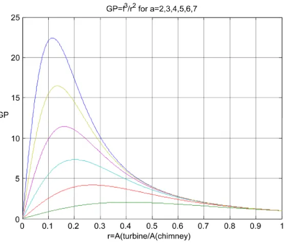
OALibJ | DOI:10.4236/oalib.1102666 5 May 2016 | Volume 3 | e2666 We define GP 12 f3
( )
rr
= as the Geometric Performance Index of the ESCP. In Figure 3 and Figure 4 the
functions f(r) and GP are shown for various a values.
As we can see by the figures GP can become several times higher than 1. For example for a reasonable esti-mation of a around 5 and a proper choice of r = 0.2, the value of GP can be as high as 11. Thus by this theory is anticipated that this ESCP can generate up to 11 times more electrical energy in comparison with an equivalent conventional solar chimney power plant of the same dimensions.
Figure 3. The saturation relation between the chimney actual air speed and maximum air speed as function of the ratio r of cross section of operating air turbine openings to chimney cross section with various values of parameter a. Upper curve means greater α.
Figure 4. The geometric performance index GP as function of r for various
values of the parameter a. Upper curve means greaterα.
0 0.1 0.2 0.3 0.4 0.5 0.6 0.7 0.8 0.9 1
0 0.2 0.4 0.6 0.8 1 1.2 1.4
r=A(turbines)/A(chimney)
f=
V
c
hi
m
ney
/V
c
hi
m
ney
,M
ax
[image:5.595.174.450.188.403.2] [image:5.595.177.455.460.697.2]OALibJ | DOI:10.4236/oalib.1102666 6 May 2016 | Volume 3 | e2666 Such an extraordinary result begs a proper justification in terms of the true physical origin of the GP factor which we attempt to provide in the next paragraphs.
Many researchers in the field of solar chimneys technology have often questioned the reasons for the ex-tremely low thermal efficiency of the conventional solar chimney power plants.
As a matter of fact the useful solar thermal power generated in the greenhouse entering at the bottom entrance of a solar chimney is given by PCh =mC P∆T, where m is the moving air mass in kg/sec, CP~1004 and ΔT
the temperature increase of the entering in the chimney air stream from the ambient air temperature.
It can be shown theoretically [9] that the maximum air speed inside the chimney is defined exclusively by the temperature difference ΔT and H, the height of the solar chimney, and is given by the relation
(
)
0
2
1 Ch
T
U gH
T k
∆ ≈
+ (6)
In (6), g = 9.81, T0 the ambient absolute temperature and k ~0.1 is a reasonable estimation for a well designed solar chimney with smooth internal surface and a ratio of height/diameter ≥8.
The maximum kinetic power of the rising air stream inside the chimney will given by 2 2
Ch
mU . Thus the electric power, generated by the turbine placed inside the chimney, should be a part of this quantity, a fact that can be expressed with the aid of an appropriate efficiency coefficient as
2 1 2
El T Ch
P =η mU (7)
The coefficient ηT expresses the overall efficiency of the turbine and electric generator hence we end up with the relation:
(
)
0 1
El T
T
P mgH
T k
η ∆
= +
(8)
From relation (8) we see that the thermal power Pth generated by the greenhouse is eventually transformed to
electricity, with an efficiency given by:
(
)
0 1
El T
th P
P gH
P =η C T +k (9)
For g ~9.81, T0 ~300 K, ηT = 0.7 and a solar chimney height of H = 200 m we end up with an estimate of the
order of PEl Pth≈0.40%. Considering furthermore that a double glassed greenhouse transforms a ~50% of the arising solar irradiation on its roof, the solar efficiency of the solar chimney technology, is in the range of ~0.2%. As a remark I mention that when a lower cost single glass greenhouse is used the efficiency drops by~33%, thus the economics of the solar chimney technology is in favor of double glass greenhouses.
The solar efficiency is defined as the electrical power generated divided by the solar irradiation on the roof of its greenhouse (or as the annual KWh of generated electricity divided by the annual solar irradiation on the roof of the greenhouse). The annual solar irradiation per m2 is a characteristic of the place of solar chimney power plant installation.
Thus we end up with a rather very low solar efficiency for an ordinary solar chimney power plant with a solar chimney height of 200 m.
This is the reason that in order to have an acceptable solar efficiency we should build solar chimneys of 1000 m (where the efficiency can become ~1.0%) and consequently accompanied by huge greenhouses due to the economics of solar chimney technology (see Appendix A). In this Appendix A, it is explained why the eco-nomics is forcing greenhouse dimensions to follow the huge dimensions of the solar chimney leading to a very expensive structure.
In order to evaluate the technical and operational feasibility and also the economic viability of the solar chimney technology we had to raise a huge and very expensive structure and spent for an experimental plant too much. If we compare this with the negligible funds in order to test PV technology or solar thermal technology made of a large number of similar units it becomes obvious why the solar chimney technology actually never tested after the Manzanares famous experimental solar chimney plant of Prof. Schlaich’s [1].
experi-OALibJ | DOI:10.4236/oalib.1102666 7 May 2016 | Volume 3 | e2666 mental power plant installed at Manzanares verified the proposed Carnot analysis. Actually the measured results were even lower due mainly to the fact that its turbine was operating without any control and thus its annual av-erage efficiency(ηT) was much lower than 0.7.
The author’s objection to all these is due to the fact that because the air turbine was installed inside the solar chimney the low solar efficiency should be expected. The ducted air turbines, for low air temperatures, can transform into rotational power only a part of the kinetic power of the air stream moving inside their duct (i.e. the solar chimney). An excellent presentation of air turbines in low temperatures is given by Wright at [3].
Thus it is the author’s opinion that the proposed Carnot cycle analysis has taken into consideration solely the internal solar chimney phenomena and not the atmospheric effects on the escaping air from the top exit of the solar chimney.
The true problem of such an approach is that in order to make the standard Carnot cycle analysis to agree with the empirical data from experimental tests, as for instance the figures shown in Prof. Schlaich’s book [1] that were obtained from a simplified analysis, one has to rely in the unjustified hypothesis that the air escaping from the chimney’s top, falls to the ground immediately after its exit.
Yet, a proper view using meteorological theory shows that this hypothesis is not true. In fact, the warm air column escaping by the solar chimney will rise up and can reach heights up to 4 km! Hence the previous Carnot model should be revised accordingly and the discrepancy should be corrected.
The hereby proposed new type of ESCP has already shown experimental indications that the efficiency can be increased say by a factor of GP ~10. In this case, an ESCP with a moderate chimney height of 200 m, could have a solar efficiency ten times higher i.e. ~2.0%. Thus with an ESCP of 200 m solar chimney we can trans-form 2.0% of the solar irradiation arriving on top of its greenhouse into electricity. The result, if proven, will give new prospects in solar chimney technology. We now suggest a possible physical explanation of this effi-ciency increase that was initially verified with a small experimental ESCP as will be presented in the next para-graph.
Several years ago an Australian company http://www.solartran.com.au/balloon_engine.htm suggested a rather unusual method for solar thermal electricity generation using uprising air balloons filled with hot air. The bal-loons could be filled with warm air made by a greenhouse and left to rise due to their atmospheric buoyancy. The balloons were then expected to reach a height at which the inside air density would approximately equal that of the ambient air at a certain height. The Australian concept was based in using ropes attached on the rising balloons to provide the mechanical energy in ground based equipment for electricity generation. The air temper-ature in the balloons of course would depend on the tempertemper-ature difference achieved by the warm air generation greenhouse of this technology.
The same buoyancy phenomenon is happening also to the escaping by the solar chimney warm air column. To provide an estimate of the height reached by this warm air column we start from a standard relation for the warm air density in zero height (https://en.wikipedia.org/wiki/Density_of_air) given as
( )
0 00 0
p T
T
RT T T
ρ ∆ = =ρ
+ ∆ (10)
where ρ0 is the ambient air density at zero height. Let us assume that the thermal losses of the warm stream dur-ing its uprisdur-ing are negligible thus the uprisdur-ing can be considered as an adiabatic process. In this case in height H
its density will become equal to ρ1
( )
H =ρ( )
∆ ⋅ −T(
1 0.0098⋅H T(
0+ ∆T)
)
2.5.This warm air density for “Aerostatic equilibrium” should become equal to the air density of the standard at-mosphere at height H given by the relationρ2
( )
H ρ0(
1 0.0065− ⋅H T0)
4.26.Using this relation we can prove that even for a temperature difference of only 20˚C we get the “Aerostatic equilibrium” at a height around 4.3 Km. Humidity effects could force the uprising stream of warm air to climb even at higher heights. The air humidity was proposed as a possible means for a solar chimney technology without solar collectors as presented in [4]. Taking into consideration “aerostatic” and humidity effects we con-sider a more realistic meteorological approach for the solar chimney power plant operation.
Similar meteorological observations justify this effect for the case of uprising warm air above the oceans. Prof. Emmanuel presented a theory explaining the strong hurricanes as due to a gigantic Carnot cycle related to warm and wet air climbing above oceans at an average height of several km see for example [5].
ad-OALibJ | DOI:10.4236/oalib.1102666 8 May 2016 | Volume 3 | e2666 ditionally exploit the escaping warm air column rising above the solar chimney. Thus we do not only use the ki-netic energy of the air stream inside the solar chimney but also part of the dynamic energy due to the rising warm air. In order to test this hypothesis a small experimental ESCP installation was constructed in central Greece.
5. The Compotades Enclosed Solar Chimney Power Plant
Near a small village in central Greece, named Compotades, a small experimental solar chimney power plant was raised a video of its operation can be viewed at http://www.youtube.com/watch?v=RVJlM6spTjU.
Its solar chimney was a light metal skeleton structure with a height of 25 m and an internal diameter of 2.5 m. The lower 15 meters of the solar chimney were permanently wrapped by a thermally insulated plastic, while the wrapping of the top was folding fabric in order to test and receive measurements with 15 m and 24 m solar chimney.
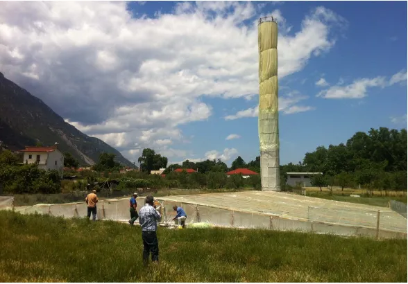
The roof of the greenhouse was made of a clear plastic and had a surface area of 1020 m2∙s depicted in the photo of Figure 5. At the entrance of the greenhouse a small turbine of 1.12 meters diameter (1 m2 cross section area) was placed as shown in Figure 6. This sole air turbine of the small power plant according to its specifi-cations had a rating power of 300 W, for an air speed of 11 m/sec, in case of incoming air stream with a speed of ~4 m/sec its output electric power drops to ~10 ÷ 15 Watts.
Figure 5. A picture of the ESCP experimental plant during measurements.
OALibJ | DOI:10.4236/oalib.1102666 9 May 2016 | Volume 3 | e2666 As can be seen from the photographic evidence this structure was a very simple form of an enclosed solar chimney power plant (ESCP) because its greenhouse was closed firmly everywhere except of one circular opening (of 1.12 m diameter) at the side opposite to its solar chimney. At this opening the air turbine generator was placed.
The air turbine forced by an incoming stream of ambient air, was rotating during daylight continuously during the period of the experiments (on June 2013) and usually was operating and a few hours after the sunset. This stream of air was becoming warmer while moving inside the greenhouse and was up-drafting through the solar chimney to upper layers of the atmosphere.
Actual implementation and measurements were completed at the small experimental ESCP for the period of June 2013.
In Table 1we present the data of June 15 2013, at 12.00. We denote with UT, the air velocity in m/sec at various
openings made at the side opposite to solar chimney (where the small turbine finally was placed) and UCh the
uprising air velocity inside the chimney for a chimney height (H) of 15 m. For a ratio of the opening area to the chimney cross section greater than one, we found an approximately constant chimney velocity of ~0.83 m/ sec.
In Table 2 we present similar measurements for an increased height of the chimney at ~24 m. Again for a ra-tio greater than one we find an approximate constant chimney air speed at ~ 1.05 m/sec.
The experimental results obtained reveal that we can definitely receive more power at the various air en-trances, in stark contrast with the predictions of the Carnot previous conservative model [1].
In fact the solar chimney maximum kinetic power for Α =Ch 5.0 m2 equals Pch= Αρ ChUCM3 2 (ρ = 1.2) which for a height of 15 m where the speed was 0.83 m/sec, gives ~1.7 W. While for the opening of 1 m2 where the respective air speed was measured at 4.0 m/sec the kinetic power calculated by Pop = Α
ρ
opUop3 2 is ~38.4 W. The respective figures from Table 2 then for a chimney height of 24 m were calculated as ~3.3 W and ~74.0 W. Thus in both cases of different chimney heights a GP higher than 20 was measured, that means that the air stream kinetic power in the turbine entrance before its placement was at least 20 times higher than the kinetic power of the rising air inside the solar chimney. This according to the classic Carnot cycle analysis [2] was not possible.Furthermore measurements were taken, after the placement of the small rotating air turbine. It is obvious that the air turbine interference could lower GP, however the electric power for the 15 m solar chimney, for the esti-mated air speed of something lower than 4m/sec in the entrance of the air turbine, as estiesti-mated by its characte-ristic output curve was a figure between 10 to 15 W. Although this result was low it was much higher than the maximum kinetic power of the rising air stream inside the chimney (~1.7 W). Such a result was also unexpected from classical solar chimney theory, giving strong experimental evidence supporting the author’s theory appli-cable in the ESCP technology.
[image:9.595.86.539.581.634.2]Thus the energy of the uprising warm air stream inside the solar chimney alone does not generate the electric-al energy of the ESCP, but the plant is supplied by a much higher amount of dynamic energy due to the atmos-phere. Thus the amount of the used energy by the ESCPs depends on atmospheric phenomena that are related in a more complicated way to the geometry of solar chimney, the greenhouse and the turbine openings of the pow-er plant.
Table 1.Solar chimney height H = 15 m, Measured air speeds at turbine and solar chimney openings for varying ratio r of their surface areas.
TT/TCh = r 0.1 0.2 0.3 0.4 0.5 1
UT m/sec 5.0 4.0 2.5 2.0 1.7 0.83
UCh m/sec 0.5 0.8 0.84 0.85 0.85 0.83
Table 2.Solar chimney height H = 24 m, Measured air speeds at turbine and solar chimney openings for varying ratio r of their surface areas.
TT/TCh = r 0.1 0.14 0.2 0.25 0.3 0.4 0.5 1
UT m/sec 6.0 6.0 5.0 4.5 4.3 3.8 3.7 1.05
[image:9.595.87.539.668.718.2]OALibJ | DOI:10.4236/oalib.1102666 10 May 2016 | Volume 3 | e2666 It is the author’s firm belief that the construction of a pilot ESCP of several KW will definitely test this new theoretical approach for the ESCP technology. This pilot ESCP could have a rating power of 18 KW and its main dimensions should be: A solar chimney H = 50 m and d = 5 m standing in the center of a single glassed hexagonal enclosed greenhouse ( as shown for example) in Figure 7, covering an area of 6000 m2.
At the perimeter’s wall of the enclosed chimney six air turbines of 1.0 m diameter and 3 KW rating power each, will be placed. The turbines openings will be equipped with electronically controlled air stop systems. The estimated cost of this DEMO ESCP will not exceed 250,000 EURO.
Measurements on this pilot ESCP will evaluate the proposed theory and the new prospects and potential of the ESCPs for solar electricity generation.
6. Water Storage Modeling of an ESCP
Thermal study of a solar chimney power plant for its overall 24 h operating cycle is a complicated mathematical problem. In references [6][7] methods of tackling this problem, taking into consideration the soil thermal sto-rage ability were presented.
In Appendix B, a detailed method is presented, in which Fourier time series analysis is used for modeling the thermal behavior during a 24 hours cycle operation of an ESCP. With the proposed method we can tackle the presence of a water storage facility that is covering a part of the base of the ESCP greenhouse.
With the proposed code we can study the effect of partial coverage (10% of its area) of the greenhouse by the water storage facility, which is the proper thermal storage method in order to leave ground space of the green-house for other symbiotic activities beneath its glassed roof. However the reader can omit the detailed reading of Appendix B without missing the main arguments and results of the present paper.
The CODE was applied to a model ESCP with main dimensions as follows: Solar chimney of 200 m height (H) and 25 m diameter (d), Circular greenhouse of ~250,000 m2 surface area (AC) and a diameter (Dc) of ~565 m, equipped with a circular concrete water storage facility of approximately ~187 m diameter and enclosed by a concrete short wall of approximately 1.1 m height and covered by a plastic cover.
The concrete structure water storage facility can be raised in the center part of the greenhouse and its water storage capacity will be ~25,000 m3. In Figure 7, the estimated daily variation of the ambient temperature and achieved temperature increase ΔT in ˚C, and its daily % variations of the horizontal solar irradiation and the % calculated power output are shown (for GP ~11, a = 5 and r = 1/5), with and without the thermal storage facility. (Table 3)
The daily results are for a typical representative day (for example an April day) of average temperature of T0 = 23˚C and a daily variation of DT= ±4˚C in a place of an annual solar irradiation WY = 2000 kWh/m2. (Figure 8)
By the Figure 8 it is evident that the ESCP, with the water thermal storage facility, operates more smoothly in comparison to the same ESCP without water thermal storage. Furthermore the rating power of the first could be 25% lower than its alternative, while both generate the same annual KWh estimated to ~11 GWh. Thus the in-crease in the construction cost of the first, due to its water thermal storage facility, is compensated by the cost increase of the second due to its higher power rating air turbines.
In order to test experimentally the water storage behavior of the proposed ESCP technology and its daily and annual electricity generation, a small demo ESCP could be constructed.
The proposed demo ESCP should be dimensioned as follows: Solar Chimney:
1) Height H = 100 m.
2) Internal diameter d = 10 m. Greenhouse:
1) Octagonal of D = ~185 m diameter. 2) Area Ac = ~24,000 m2.
3) Double glass roof of > 2% inclination, entrance height ~3 m central height ~5 m.
Internal Water Storage Facility of ~60 m diameter, enclosed by a wall of 1.2 m with a water capacity of ~3000 m3, covered by a plastic cup.
Air Turbines:
OALibJ | DOI:10.4236/oalib.1102666 11 May 2016 | Volume 3 | e2666 3) 16 electro-mechanically controlled air barriers of the openings.
The estimated construction cost of this demo ESCP reaches approximately 1.6 million EURO analyzed as shown in Table 3. This demo ESCP can be installed in any place with an obvious preference for a sunny place of annual solar irradiation ~2000 KWh/m2.
[image:11.595.162.470.169.286.2]The electric generators of this demo ESPC can be connected to a nearby electric grid thus proper induction generators should be used.
Figure 7. An initial figure of the proposed small demo of 18 KW.
Figure 8. Daily operation in an April day of an ESCP with thermal storage covering
~10% of its ground with 1 m water and without water thermal storage.
Table 3.Dimensions and construction cost figures of the Model ESCP.
Greenhouse 24000 m2 × 25 EUR/m2 600,000 EUR
Water Storage 3000 m2 × 20 EUR/m2 60,000 EUR
Solar Chimney ~160 EUR/m2 600,000 EUR
Air Turbines 16 p × 15,000 EUR/m2 240,000 EUR
Unforeseen 200,000 EUR
[image:11.595.162.468.317.572.2] [image:11.595.158.469.624.720.2]OALibJ | DOI:10.4236/oalib.1102666 12 May 2016 | Volume 3 | e2666 If no electric grid is present the demo ESCP can be operated as a local autonomous power plant in which case its electric generators should be synchronous and their output loads could be for instance ohmic resistances giv-ing their generated thermal energy to nearby water tanks
7. Conclusions
The presented ESCP technology already tested in a small experimental power plant in Greece could be a major player in renewable technology market after its successful testing with relatively low cost demonstration plants. The ESCP technology can combine low levelized cost of electricity with smooth 24 hours/day operation for 365 days/year.
The ESCP technology also has the following benefits in relation to its major competitive technologies (wind and PV and CSP):
• No water consumption;
• Zero effect on living nature and ambient;
• Local manufacturing and use of common material (steel, glass, concrete and conventional axial fans as air turbines);
• Easy and low cost maintenance;
• Longer operating life up to 50 years (its solar chimney up to 100 years);
• Their empty protected surface area beneath the glassed roofs of their greenhouses can be used partially for agriculture and or placement of parabolic trough mirrors for desalination.
References
[1] Schlaich, J. (1995) The Solar Chimney: Electricity from the Sun. Axel Mengers Edition, Stuttgart.
[2] Gannon, A. and Von Backstrom, T. (2000) Solar Chimney Cycle Analysis with System loss and solar Collector Per-formance. Journal of Solar Energy Engineering, 122, 133-137.
[3] Wright, T. (1999) Fluid Machinery, Performance Analysis and Design. CRC Press.
[4] Papageorgiou, C.D., Psalidas, M. and Katopodis, P. (2010) Solar Chimney Technology without Solar Collectors. SCPT
2010 Solar Chimney Power Technology International Conference, Bochum, Germany, 28-30 September 2010, 275- 282.
[5] Emanuel, K.A. (1986) An Air-Sea Interaction Theory for Tropical Cyclones. Part I: Steady State Maintenance. Journal of the Atmospheric Sciences, 43, 585-604. http://dx.doi.org/10.1175/1520-0469(1986)043<0585:aasitf>2.0.co;2
[6] dos S. Bernades, M.A., Vob, A. and Weinrebe, G. (2003) Thermal and Technical Analyses of Solar Chimneys. Solar Energy, 75, 511-524. http://dx.doi.org/10.1016/j.solener.2003.09.012
[7] Pretorius, J.P. and Kroger, D.G. (2006) Solar Chimney Power Plant Performance. Journal of Solar Energy Engineering,
128, 302-311.
[8] Gengel, Y.A. (1998) Heat Transfer. McGraw Hill, New York.
OALibJ | DOI:10.4236/oalib.1102666 13 May 2016 | Volume 3 | e2666
Appendix A: Cost Optimization of the Solar Chimney Technology
Let us consider a Solar Chimney Power Plant (SCPP) generating annually a certain amount of electricity in KWh defined by the symbol W, and made of three major parts:
• A Solar Chimney of height H and an average internal diameter d
For stability reasons we assume that d =C2⋅H • A circular Greenhouse of area Ac
• An electricity generating system of air turbines of rating power P = W/h (h = 8760 X the capacity factor of the technology)
The basic construction costs of the three main parts are approximately given by the relations:
SCC = Solar Chimney Cost = C H d1⋅ ⋅ =C C1⋅ 2⋅H2 GHC = Greenhouse cost = C3⋅AC
ATC = Air Turbine cost = C4⋅ =P C4⋅W h
Thus the overall SCPP cost (TC) is equal to the following sum
(
2)
(
)
1 2 3 4 1
TC= C C⋅ ⋅H +C ⋅Ac+C W h⋅ ⋅ +ε where ε represents the overhead and unforeseen costs. Ac-cording to previous presented theory W =C5⋅AC⋅H We may take a constant W and ask under what condition
TC is minimized. In order TC to be minimum the sum C C1⋅ 2⋅H2+C3⋅Ac should also be minimized. Replacing
(
5)
C
A = W C H the following function of H should be minimized f H
( )
=C C1⋅ 2⋅H2+C3⋅(
W C5)
H,1, 2, 3, 4, 5
C C C C C are independent of H
From the above one obtains
(
)
21 2 3 5
0 2 0
f H C C H C W C H
∂ ∂ = ⇒ ⋅ ⋅ ⋅ − ⋅ = or 2⋅C C1⋅ 2⋅H2=C3⋅
(
W C5)
Hi.e. GHC= ⋅2 SCC
Conclusively, in order to minimize the construction cost for constant annual KWh generation of a solar chimney power plant, its greenhouse cost should be approximately twice the cost of its solar chimney.
Appendix B: ESCP Thermal Heat Transfer Analysis
1. The ESCP Model
The ESCP model with a circular collector is shown in the indicative diagram in Figure B1. The circular solar collector of this ESCP is divided in a series of M circular sectors of equal width Δr as shown in Figure B1.
Water(height dh)
Δr
r
Tin Tout
Hin
Hout
hl
Cover
Curtain
hup
hin
hw
Horizontal Solar irradiance G
Tc
Tw
Tsk
To
Wind (υw)
hrcw
hrsk
hrsc
dh
[image:13.595.115.512.466.706.2]Ts
OALibJ | DOI:10.4236/oalib.1102666 14 May 2016 | Volume 3 | e2666 The mth circular sector (m = 1 to M) will have a width ∆ =r
(
Dc−Din)
M , an average radius(
1)
2 1 2
m c
r =D − ∆ ⋅r m − and an average height Hm =
(
Hin m, +Hex m,)
2. For a linear variation of the roof height Hm=Hin+(
Hout−Hin) (
⋅ m−1 2)
M, where: Dc = solar collector diameter and Din = Final internaldiameter of the solar collector. If not available data are given Din≈ 2∙d.
These consecutive circular sectors, for the moving stream of air of mass flow m, are special tubes of almost parallel flat surfaces and an equivalent diameters de m, = ∗2 Hm. The ambient air as moving towards the en-trance of the first circular sector is assumed that it is increasing its temperature T0 to T0 + dT .The exit tempera-ture of the first sector is the inlet temperatempera-ture for the second etc. and finally the exit temperatempera-ture of the final Mth sector is the T03, i.e. the inlet temperature to the air turbines.
The mth circular sector (m = 1 to M) will have a width ∆ =r
(
Dc−Din)
M , an average radius(
1)
2 1 2
m c
r =D − ∆ ⋅r m − and an average height Hm =
(
Hin m, +Hex m,)
2.For a linear variation of the roof height Hm=Hin+
(
Hout−Hin) (
⋅ m−1 2)
M, where: Dc = solar collectordiameter and Din= Final internal diameter of the solar collector. If not available data are given Din≈ 2∙d.
These consecutive circular sectors, for the moving stream of air of mass flow m, are special tubes of almost parallel flat surfaces and an equivalent diameters de m, = ∗2 Hm.
The ambient air as moving towards the entrance of the first circular sector is assumed that it is increasing its temperature T0 to T0 + dT.
The exit temperature of the first sector is the inlet temperature for the second etc. and finally the exit temper-ature of the final Mth sector is the T03, i.e. the inlet temperature to the air turbines.
2. Daily Variations of Ambient and Sky Temperature and Solar Irradiation
The ambient (T0) and sky (Tsk) temperatures are in general functions of time. If there are not sufficient data for a
place of ESCP installation the following formulae in ˚C and t in hours from midnight can be used for the aver-age annual representation day:
( )
(
0.1463sin(
(
11)
π 6)
0.9756 sin(
(
11)
π 12)
)
o o o
T t =T + ∆ ⋅T t− + t−
For the average day if not available data, T0 = 20˚C.
( )
( )
0.711 0.0056( )
0.000073 2( )
0.013 cos π 1 4 12SK o dp dp
t T t =T t ⋅ + ⋅T t + ⋅T t + ⋅ ⋅
as given by Bernades M.A. dos
S., Vob A., Weinrebe G. in [6].
where Tdp(t) is the due point temperature in ˚C given approximately by the formula:
( )
100273.15
5
dp o
RH
T ≈T t − − − , where RH is the relative humidity of the ambient air %. Without any avail-
able data, RH can be assumed to be equal in average to 50%, i.e. in average Tdp(t) = T0(t)− 10 in ˚C.
The solar irradiation on horizontal surface is a very important characteristic of the place of SCPP’s installa-tion. The annual solar irradiation per m2 on horizontal surface Wy is a characteristic figure of the place and
should be given or estimated approximately by existing solar maps. The average horizontal solar irradiance on the sector roof is equal to the annual solar irradiation divided by 8760 hours. However for the average represen-tation day of the year, if other data are not available, the horizontal solar irradiance G(t) can be assumed as a si-nusoidal function of time between the 6th and the 18th hour and zero outside, hence:
( )
cos(
(
12)
π 12)
6 180 0 6,18 24
M
G t t
G t
t t
⋅ − ⋅ ≤ ≤
=
< < < <
where: GM = π∙Wy/8760. If data are available T0(t), Tdp(t), Tsk(t), G(t) can be described by their real equivalent
daily functions for the representative average day of the year or any other day. As representation day usually is received the day of which its calculated daily electrical energy production is equal in approximation to the aver-age daily electrical energy. Thus the annual electricity production by the ESCP will be 365 times this averaver-age daily electricity production. As a general rule an April the day’s duration is very close to the average representa-tion day. The solar irradiarepresenta-tion energy per m2 arriving on the ground of the sector is given approximately by
ta∙G(t), where ta is the mixed coefficient {overall covers transmissivity ground absorptivity} for short
OALibJ | DOI:10.4236/oalib.1102666 15 May 2016 | Volume 3 | e2666 transmissivity is estimated to 0.9 while for two covers is estimated to 0.81. The absorptivity for treated ground if data are not available is estimated to 0.9.
Without any available data, RH can be received as equal in average to 50%, i.e. in average Tdp(t) = T0(t) − 10 in ˚C.
The solar irradiation on horizontal surface is a very important characteristic of the place of SCPP’s installa-tion. The annual solar irradiation per m2 on horizontal surface Wy is a characteristic figure of the place and
should be given or estimated approximately by existing solar maps. The average horizontal solar irradiance on the sector roof is equal to the annual solar irradiation divided by 8760 hours. However for the average represen-tation day of the year, if other data are not available, the horizontal solar irradiance G(t) can be assumed as a si-nusoidal function of time between the 6th and the18th hour and zero outside. Thus:
( )
cos(
(
12)
π 12)
6 180 0 6,18 24
M
G t t
G t
t t
⋅ − ⋅ ≤ ≤
=
< < < <
where: GM= π∙Wy/8760.
If data are available T0(t), Tdp(t), Tsk(t), G(t) can be described by their real equivalent daily functions for the
representative average day of the year or any other day. As representation day usually is received the day of which its calculated daily electrical energy production is equal in approximation to the average daily electrical energy. Thus the annual electricity production by the ESCP will be 365 times this average daily electricity pro-duction. As a general rule an April day is very close to the average representation day. The solar irradiation energy per m2 arriving on the ground of the sector is given approximately by t G ta
( )
, where tais the mixedcoefficient {overall covers transmissivity ground absorptivity} for short wavelength solar light irradiation. If data are not available for the cover and curtain for one cover, the overall transmissivity is estimated to 0.9 while for two covers is estimated to 0.81. The absorptivity for treated ground if data are not available is estimated to 0.9.
3. Heat Transfer Analysis of the Basic Two Glazing Model
The mass flow m of the sector could be varying during the daily cycle or constant. In the present analysis the mass flow is considered constant, as the value that gives to the ESCP its maximum electricity generation. An in-itial estimation for m is
(
π 2)
4
m = ⋅ ⋅ρ υ ⋅d , where air speed is υ is estimated to 7 - 8 m/sec and the air
den-sity given by ρ = p0/(287 × 307.15). The internal solar chimney diameter is constant and equal to d.
Following the circular sector diagram for a double glazing solar collector, as shown in Figure 2, the following equations are derived:
• For outer cover (w), hw⋅
(
Tw−To)
+hrsk⋅(
Tw−Tsk)
=hcw⋅(
Tc−Tw)
where: hcw=hin+hrcw • For inner cover or curtain (c), hcw⋅(
Tc−Tw)
=hur⋅(
T−Tc)
+hrsc⋅(
Ts−Tc)
• For the moving air, hair⋅
(
T−Tin)
= ⋅hl(
Ts−T)
−hup⋅(
T−Tc)
where:(
)
1
, ,
π 2 2
p out in
air in out in
m c T T
h T T T T T
r r
⋅ +
= = − = −
⋅ ⋅ ∆
• For ground surface (s) qgr=tα⋅G t
( )
− ⋅hl(
Ts −T)
−hrsc⋅(
Ts−Tc)
where qgr is the heat power going down to the ground.The first three equations form a linear system as follows:
(
)
(
)
(
)
0
0
w rsk cw w cw c cw o rsk sk
cw w cw up rsc c up rsc s
w up c air l up air in l s
h h h T h T T h T h T
h T h h h T h T h T
T h T h h h T h T h T
+ + ⋅ − ⋅ + ⋅ = ⋅ + ⋅
− ⋅ + + + ⋅ − ⋅ = ⋅
⋅ − ⋅ + + + ⋅ = ⋅ + ⋅
Through of which the temperatures or outer cover Tw, of the curtain Tc and the air T can be expressed as linear
functions of the ground temperatures Ts. and the irradiance G are functions of time given in the previous
para-graph. These linear forms are in general in the form:
1 2, 3 4, 5 6
c s s w s
T = ⋅ +c T c T =c T⋅ +c T =c ⋅ +T c ,
OALibJ | DOI:10.4236/oalib.1102666 16 May 2016 | Volume 3 | e2666 Replacing Tcand Tin the ground equation: qgr =tα⋅G t
( )
− ⋅hl(
Ts −T)
−hrsc⋅(
Ts −Tc)
The following relation is derived
( )
( ) ( ) ( )
gr s
q t =q t −h t ⋅T t ,
where
( )
(
)
(
)
( )
( )
3 1
4 2
1 1 ,
l rsc
l rsc
h t h c h c
q t tα G t h c h c
= ⋅ − + ⋅ −
= ⋅ + ⋅ + ⋅
We can always write for each cover and the moving air a similar number of linear relations between the tem-peratures with heat transfer parameters as coefficients and always we can solve the linear system in order to de-rive a relation for the ground surface (s), connecting the ground temperature Ts the power heat flow down to the
ground surface qgr. In general all the functions appearing on the ground relation are functions of time (t). In
or-der to calculate the time functions Ts(t) and qgr(t) it is necessary to have one more relation between them. This
relation it will be derived by the ground heat flow partial differential equations as explained in the next paragraph.
4. Ground Equivalent Equation in Fourier Space
The ground bellow the sector is considered as infinitely wide thus the surface temperature it depends in the depth distance (z) and time (t). It is also considered homogeneous and characterized by three parameters, its density ρgr, its specific heat capacity cgr and its thermal conductivity kgr. The ground partial differential equations,
relating the surface temperature Ts(z,t) and the down-moving heat power qg(z,t), starting from its surface (z = 0) and
going down (see Figure 2), can be written as the following set of two equations:
( )
( )
( )
( )
, 1 , , , s gr gr gr s gr gr T z tq z t
z k
q z t T z t
c
z ρ t
∂ = − ⋅ ∂ ∂ ∂ = − ⋅ ⋅ ∂ ∂ where qgr(z) for z → ∞ is zero.
Let us consider that Ts(z,t) and qg(z,t) are sinusoidal functions of time as follows:
( )
,( )
ej t, gr( )
, gr( )
ej tT z t =T z ⋅ ⋅ ⋅ω q z t =q z ⋅ ⋅ ⋅ω
Thus the set of two differential equations becomes:
( )
( )
( )
( )
1 s gr gr grgr gr s T z
q z
z k
q z
j c T z
z ω ρ
∂ = − ⋅ ∂ ∂ = − ⋅ ⋅ ⋅ ⋅ ∂
This set represents an infinite homogeneous transmission line with “equivalent voltage” the function Ts(z) and
“equivalent current” the function qgr(z).
According to transmission line theory this infinite transmission line is equivalent to its admittance defined by the relation: Y = j⋅ ⋅ω ρ
(
gr⋅cgr⋅kgr)
.Thus the Fourier transform of heat flow qgr for z = 0, is related to the Fourier transform of the Ground
temper-ature Ts in the surface z = 0 by the linear relation:
gr s s gr gr gr
q =T Y⋅ =T ⋅ j⋅ ⋅ω k ⋅ρ ⋅c
For the daily variation the ground temperature in z = 0, Ts(t) can be analysed in a Fourier series with a
funda-mental harmonic ω0 = 2 × π/(24 × 60 × 60) as follows:
( )
2(
)
2
, e o , ,
M
j n t
s s n s n s n
n M
T t T ⋅ ⋅ ⋅ω T T∗
=−
=
∑
⋅ =For each harmonic the previous is valid for ω = n∙ω0 thus:
,
gr n n n n o gr gr gr
OALibJ | DOI:10.4236/oalib.1102666 17 May 2016 | Volume 3 | e2666 In order to take into consideration the water thermal storage effect, let us assume that the equivalent water height dh is very small, with an assumed very high thermal conductivity thus its temperatures in both of its sur-faces are almost equal to the ground temperature Ts. Under these reasonable approximations the water thermal
storage sheet of thickness dh is equivalent in Fourier space to an admittance
w w
Y = ⋅j dh c⋅ ⋅ω, where cw= water specific heat = 4,186,800.
Thus in case of ground plus artificial water thermal storage of equivalent height dh the linear relation for the Fourier transform harmonics of temperature Tsand heat flow qgrare given by the relation: qgr n, =T Yn⋅ n Where:
(
)
n o gr gr gr w o
Y = j n⋅ ⋅ω ⋅ ρ ⋅c ⋅k + ⋅j dh C⋅ ⋅ ⋅n ω .
5. Fourier Analysis of the Sector
On the ground surface (s) the time equation relating the ground temperature Ts(t) and the power heat transfer to
the ground qgr(t) is given by the equation:
( )
( ) ( ) ( )
gr s
q t =q t −h t ⋅T t
In the equation two known functions q(t) and h(t) appear. These functions can be expressed by the following Fourier series:
( )
2(
)
2 e M
j n t
n n n
n M
q t q ⋅ ⋅ ⋅ωο q q∗
=−
=
∑
⋅ = ,( )
2(
)
2 e M
jn t
n n n
n M
h t h ωο h h∗
=−
=
∑
⋅ =While the Fourier series of the function qgr(t) is given below where the Fourier harmonics of the function qgr(t)
have been replaced by the harmonics of the Ts(t).
( )
2 22 2
, e , e
M M
j n t j n t
gr gr n s n n
n M n M
q t q ⋅ ⋅ ⋅ωο T Y ⋅ ⋅ ⋅ωο
=− =−
=
∑
⋅ =∑
⋅ ⋅We can replace the functions with their Fourier series from −M2 up to M2 harmonic, in the ground relation
( )
( ) ( ) ( )
gr s
q t =q t −h t ⋅T t . The bilinear form of the produced equation is equivalent to a set of 2 × M2 + 1 linear relations. The equations are derived equating the coefficients of the time functions exp(j∙n∙ω0∙t) for −Μ2≤ n≤ +M2 and considering the coefficients of these functions negligible for n > M2 and n < −M2. This is a very rea-sonable estimation due to the fact that the harmonics of all time functions are rapidly decreasing.
For example for M2 = 2 the following matrix equation it is the set of relevant equations:
, 2
0 2 1 2 2
, 1
1 0 1 1 2 1
,0
2 1 0 0 1 2 0
,1
2 1 0 1 1 1
,2
2 1 0 2 2
0 0 0 0 0 0 s s s s s T
h Y h h q
T
h h Y h h q
T
h h h Y h h q
T
h h h Y h q
T
h h h Y q
− − − − − − − − − − − − − + + + = + +
The matrix equation can be solved and Ts,n can be calculated for −Μ2≤ n≤ +M2. Thus Ts(t) can be calculated by its Fourier time series as follows:
( )
22
,
,0 e o
M
j n t s n
s s
n M
T t T Real T
ο ω ⋅ ⋅ ⋅ =− = + ⋅
∑
It is suggested to use the Real part operator, before the Fourier sum, in order to get rid of the negligible im-aginary parts due to computer and method approximations.
Usually it is enough to calculate N values of the previous function for: t=
(
ν−1)
N×24 60 60× × i.e.(
)
0 t 2 π 1 N
ω ⋅ = ⋅ ⋅ν − for 1 ≤ ν < N. Using the linear relations connecting Tw(t), Tc(t) and T(t) with Ts(t) these
temperature time functions can be for the same time sequence.
The temperature dependent heat transfer coefficients can be re estimated and the same program can be run again defining the temperatures with a better accuracy etc. (usually two to three times running is enough).
ac-OALibJ | DOI:10.4236/oalib.1102666 18 May 2016 | Volume 3 | e2666 ceptable accuracy in T03(t)calculation.
Thus using an approximate proportion coefficient relating the heat Power output (defined by m Cp⋅ ⋅ ∆T ) of the greenhouse as function of time for 24 hours daily period the Electric Power output can be calculated. The code can be used to calculate the best daily average value for the average daily mass flow m in order to max-imize the power output of the ESCP. Using control methods through the openings we can vary this average mass flow during the 24 hours daily period in order to achieve an optimal performance of the ESCP.