Stock Price Prediction using Long Short Term Memory

(1)

Stock Price Prediction Using Long Short Term Memory

Raghav Nandakumar

1

_{, Uttamraj K R}

2

_{, Vishal R}

3

_{, Y V Lokeswari}

4

1,2,3_{Department of Computer Science and Engineering; SSN College of Engineering;} Chennai, Tamil Nadu, India

4_{Assistant Professor; Department of Computer Science and Engineering; SSN College of Engineering;} Chennai, Tamil Nadu, India

---*---Abstract -**

Predicting stock market prices is a complex task that traditionally involves extensive human-computer interaction. Due to the correlated nature of stock prices, conventional batch processing methods cannot be utilized efficiently for stock market analysis. We propose an online learning algorithm that utilizes a kind of recurrent neural network (RNN) called Long Short Term Memory (LSTM), where the weights are adjusted for individual data points using stochastic gradient descent. This will provide more accurate results when compared to existing stock price prediction algorithms. The network is trained and evaluated for accuracy with various sizes of data, and the results are tabulated. A comparison with respect to accuracy is then performed against an Artificial Neural Network.

Key Words:stock prediction, Long Short Term Memory, Recurrent Neural Network, online learning, stochastic gradient descent

1. INTRODUCTION

The stock market is a vast array of investors and traders who buy and sell stock, pushing the price up or down. The prices of stocks are governed by the principles of demand and supply, and the ultimate goal of buying shares is to make money by buying stocks in companies whose perceived value (i.e., share price) is expected to rise. Stock markets are closely linked with the world of economics — the rise and fall of share prices can be traced back to some Key Performance Indicators (KPI's). The five most commonly used KPI's are the opening stock price (`Open'), end-of-day price (`Close'), intra-day low price (`Low'), intra-intra-day peak price (`High'), and total volume of stocks traded during the day (`Volume').

Economics and stock prices are mainly reliant upon subjective perceptions about the stock market. It is near-impossible to predict stock prices to the T, owing to the volatility of factors that play a major role in the movement of prices. However, it is possible to make an educated estimate of prices. Stock prices never vary in isolation: the movement of one tends to have an avalanche effect on several other stocks as well [2]. This aspect of stock price movement can be used as an important tool to predict the prices of many stocks at once. Due to the sheer volume of money involved and number of transactions that take place every minute, there comes a trade-off between the accuracy and the volume of predictions made; as such, most stock prediction

systems are implemented in a distributed, parallelized fashion [7]. These are some of the considerations and challenges faced in stock market analysis.

2. LITERATURE SURVEY

The initial focus of our literature survey was to explore generic online learning algorithms and see if they could be adapted to our use case i.e., working on real-time stock price data. These included Online AUC Maximization [8], Online Transfer Learning [9], and Online Feature Selection [1]. However, as we were unable to find any potential adaptation of these for stock price prediction, we then decided to look at the existing systems [2], analyze the major drawbacks of the same, and see if we could improve upon them. We zeroed in on the correlation between stock data (in the form of dynamic, long-term temporal dependencies between stock prices) as the key issue that we wished to solve. A brief search of generic solutions to the above problem led us to RNN’s [4] and LSTM [3]. After deciding to use an LSTM neural network to perform stock prediction, we consulted a number of papers to study the concept of gradient descent and its various types. We concluded our literature survey by looking at how gradient descent can be used to tune the weights of an LSTM network [5] and how this process can be optimized. [6]

3. EXISTING SYSTEMS AND THEIR DRAWBACKS

(2)

An alternative approach to stock market analysis is to reduce the dimensionality of the input data [2] and apply feature selection algorithms to shortlist a core set of features (such as GDP, oil price, inflation rate, etc.) that have the greatest impact on stock prices or currency exchange rates across markets [10]. However, this method does not consider long-term trading strategies as it fails to take the entire history of trends into account; furthermore, there is no provision for outlier detection.

4. PROPOSED SYSTEM

We propose an online learning algorithm for predicting the end-of-day price of a given stock (see Figure 2) with the help of Long Short Term Memory (LSTM), a type of Recurrent Neural Network (RNN).

4.1 Batch versus online learning algorithms

Online and batch learning algorithms differ in the way in which they operate. In an online algorithm, it is possible to stop the optimization process in the middle of a learning run and still train an effective model. This is particularly useful for very large data sets (such as stock price datasets) when the convergence can be measured and learning can be quit early. The stochastic learning paradigm is ideally used for online learning because the model is trained on every data point — each parameter update only uses a single randomly chosen data point, and while oscillations may be observed, the weights eventually converge to the same optimal value. On the other hand, batch algorithms keep the system weights constant while computing the error associated with each sample in the input. That is, each parameter update involves a scan of the entire dataset — this can be highly time-consuming for large-sized stock price data. Speed and accuracy are equally important in predicting trends in stock price movement, where prices can fluctuate wildly within the span of a day. As such, an online learning approach is better for stock price prediction.

[image:2.595.39.284.577.749.2]

4.2 LSTM – an overview

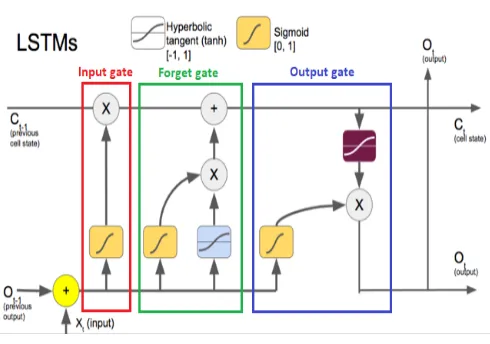
Fig - 1: An LSTM memory cell

LSTM's are a special subset of RNN’s that can capture context-specific temporal dependencies for long periods of time. Each LSTM neuron is a memory cell that can store other information i.e., it maintains its own cell state. While neurons in normal RNN’s merely take in their previous hidden state and the current input to output a new hidden state, an LSTM neuron also takes in its old cell state and outputs its new cell state.

An LSTM memory cell, as depicted in Figure 1, has the following three components, or gates:

1. Forget gate: the forget gate decides when specific portions of the cell state are to be replaced with more recent information. It outputs values close to 1 for parts of the cell state that should be retained, and zero for values that should be neglected.

2. Input gate : based on the input (i.e., previous output o(t-1), input x(t), and previous cell state c(t-1)), this section of the network learns the conditions under which any information should be stored (or updated) in the cell state

3. Output gate: depending on the input and cell state, this portion decides what information is propagated forward (i.e., output o(t) and cell state c(t)) to the next node in the network.

Thus, LSTM networks are ideal for exploring how variation in one stock's price can affect the prices of several other stocks over a long period of time. They can also decide (in a dynamic fashion) for how long information about specific past trends in stock price movement needs to be retained in order to more accurately predict future trends in the variation of stock prices.

4.3 Advantages of LSTM

The main advantage of an LSTM is its ability to learn context-specific temporal dependence. Each LSTM unit remembers information for either a long or a short period of time (hence the name) without explicitly using an activation function within the recurrent components.

(3)

Additionally, LSTM’s are also relatively insensitive to gaps (i.e., time lags between input data points) compared to other RNN’s.

4.4 Stock prediction algorithm

Fig - 2: Stock prediction algorithm using LSTM

4.5 Terminologies used

Given below is a brief summary of the various terminologies relating to our proposed stock prediction system:

1. Training set : subsection of the original data that is used to train the neural network model for predicting the output values

2. Test set : part of the original data that is used to make predictions of the output value, which are then compared with the actual values to evaluate the performance of the model

3. Validation set : portion of the original data that is used to tune the parameters of the neural network model

4. Activation function: in a neural network, the activation function of a node defines the output of that node as a weighted sum of inputs.

Here, the sigmoid and ReLU (Rectified Linear Unit) activation functions were tested to optimize the prediction model.

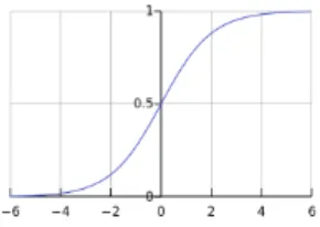
a. Sigmoid – has the following formula

[image:3.595.378.523.181.284.2]

and graphical representation (see Figure 3)

Fig - 3: sigmoid activation function

b. ReLU – has the following formula

and graphical representation (see Figure 4)

Fig - 4: ReLU activation function

5. Batch size : number of samples that must be processed by the model before updating the weights of the parameters

6. Epoch : a complete pass through the given dataset by the training algorithm

7. Dropout: a technique where randomly selected neurons are ignored during training i.e., they are “dropped out” randomly. Thus, their contribution to the activation of downstream neurons is temporally removed on the forward pass, and any weight updates are not applied to the neuron on the backward pass.

(4)

9. Cost function: a sum of loss functions over the training set. An example is the Mean Squared Error (MSE), which is mathematically explained as follows:

10. Root Mean Square Error (RMSE): measure of the difference between values predicted by a model and the values actually observed. It is calculated by taking the summation of the squares of the differences between the predicted value and actual value, and dividing it by the number of samples. It is mathematically expressed as follows:

In general, smaller the RMSE value, greater the accuracy of the predictions made.

[image:4.595.317.555.73.216.2]

5. OVERALL SYSTEM ARCHITECTURE

Fig – 5: LSTM-based stock price prediction system

The stock prediction system depicted in Figure 5 has three main components. A brief explanation of each is given below:

[image:4.595.48.273.401.597.2]

5.1 Obtaining dataset and preprocessing

Fig – 6: Data preprocessing

Benchmark stock market data (for end-of-day prices of various ticker symbols i.e., companies) was obtained from two primary sources: Yahoo Finance and Google Finance. These two websites offer URL-based APIs from which historical stock data for various companies can be obtained for various companies by simply specifying some parameters in the URL.

The obtained data contained five features:

1. Date: of the observation 2. Opening price: of the stock

3. High: highest intra-day price reached by the stock 4. Low: lowest intra-day price reached by the stock 5. Volume: number of shares or contracts bought and

sold in the market during the day

6. OpenInt i.e., Open Interest: how many futures contracts are currently outstanding in the market

The above data was then transformed (Figure 6) into a format suitable for use with our prediction model by performing the following steps:

1. Transformation of time-series data into input-output components for supervised learning

2. Scaling the data to the [-1, +1] range

5.2 Construction of prediction model

[image:4.595.310.556.584.722.2]

(5)

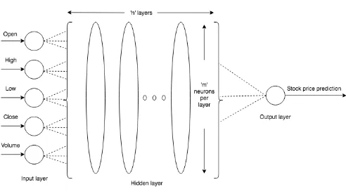
The input data is split into training and test datasets; our LSTM model will be fit on the training dataset, and the accuracy of the fit will be evaluated on the test dataset. The LSTM network (Figure 7) is constructed with one input layer having five neurons, 'n' hidden layers (with 'm' LSTM memory cells per layer), and one output layer (with one neuron). After fitting the model on the training dataset, hyper-parameter tuning is done using the validation set to choose the optimal values of parameters such as the number of hidden layers 'n', number of neurons 'm' per hidden layer, batch size, etc.

5.3 Predictions and accuracy

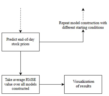
Fig – 8: Prediction of end-of-day stock prices

Once the LSTM model is fit to the training data, it can be used to predict the end-of-day stock price of an arbitrary stock.

This prediction can be performed in two ways:

1. Static – a simple, less accurate method where the model is fit on all the training data. Each new time step is then predicted one at a time from test data. 2. Dynamic – a complex, more accurate approach

where the model is refit for each time step of the test data as new observations are made available.

The accuracy of the prediction model can then be estimated robustly using the RMSE (Root Mean Squared Error) metric. This is due to the fact that neural networks in general (including LSTM) tend to give different results with different starting conditions on the same data.

We then repeat the model construction and prediction several times (with different starting conditions) and then take the average RMSE as an indication of how well our configuration would be expected to perform on unseen real-world stock data (figure 8). That is, we will compare our predictions with actual trends in stock price movement that can be inferred from historical data.

6. VISUALIZATION OF RESULTS

[image:5.595.309.542.178.356.2]

Figure 9 shows the actual and the predicted closing stock price of the company Alcoa Corp, a large-sized stock. The model was trained with a batch size of 512 and 50 epochs, and the predictions made closely matched the actual stock prices, as observed in the graph.

[image:5.595.64.249.243.406.2]

Fig - 9: Predicted stock price for Alcoa Corp

Figure 10 shows the actual and the predicted closing stock price of the company Carnival Corp, a medium-sized stock. The model was trained with a batch size of 256 and 50 epochs, and the predictions made closely matched the actual stock prices, as observed in the graph.

Fig - 10: Predicted stock price for Carnival Corp

[image:5.595.314.534.469.654.2]

(6)

[image:6.595.42.274.93.275.2]

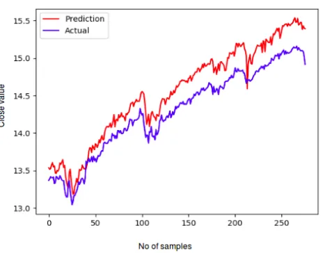
Fig - 11: Predicted stock price for DH Goodman Corp

We can thus infer from the results that in general, the prediction accuracy of the LSTM model improves with increase in the size of the dataset.

7. COMPARISON OF LSTM WITH ANN

The performance of our proposed stock prediction system, which uses an LSTM model, was compared with a simple Artificial Neural Network (ANN) model on five different stocks of varying sizes of data.

Three categories of stock were chosen depending upon the size of data set. Small data set is a stock for which only about 10 years of data is available e.g., Dixon Hughes. A medium-sized data set is a stock for which data up to 25 years is available, with examples including Cooper Tire & Rubber and PNC Financial. Similarly, a large data set is one for which more than 25 years of stock data is available; Citigroup and American Airlines are ideal examples of the same.

Parameters such as the training split, dropout, number of layers, number of neurons, and activation function remained the same for all data sets for both LSTM and ANN. Training split was set to 0.9, dropout was set to 0.3, number of layers was set to 3, number of neurons per layer was set to 256, the sigmoid activation function was used, and the number of epochs was set to 50. The batch sizes, however, varied according to the stock size. Small datasets had a batch size of 32, medium-sized datasets had a batch size of 256, and large datasets had a batch size of 512.

Table - 1: Comparison of error rates from the LSTM and

ANN models

Data Size Stock Name LSTM

(RMSE) (RMSE) ANN

Small Dixon

Hughes 0.04 0.17

Medium Cooper Tire

& Rubber 0.25 0.35

Medium PNC

Financial 0.2 0.28

Large CitiGroup 0.02 0.04

Large Alcoa Corp 0.02 0.04

In Table 1, the LSTM model gave an RMSE (Root Mean Squared Error) value of 0.04, while the ANN model gave 0.17 for Dixon Hughes. For Cooper Tire & Rubber, LSTM gave an RMSE of 0.25 and ANN gave 0.35. For PNC Financial, the corresponding RMSE values were 0.2 and 0.28 respectively. For Citigroup, LSTM gave an RMSE of 0.02 and ANN gave 0.04, while for American Airlines, LSTM gave an RMSE of 0.02 and ANN gave 0.04.

7. CONCLUSION AND FUTURE WORK

The results of comparison between Long Short Term Memory (LSTM) and Artificial Neural Network (ANN) show that LSTM has a better prediction accuracy than ANN.

Stock markets are hard to monitor and require plenty of context when trying to interpret the movement and predict prices. In ANN, each hidden node is simply a node with a single activation function, while in LSTM, each node is a memory cell that can store contextual information. As such, LSTMs perform better as they are able to keep track of the context-specific temporal dependencies between stock prices for a longer period of time while performing predictions.

An analysis of the results also indicates that both models give better accuracy when the size of the dataset increases. With more data, more patterns can be fleshed out by the model, and the weights of the layers can be better adjusted.

At its core, the stock market is a reflection of human emotions. Pure number crunching and analysis have their limitations; a possible extension of this stock prediction system would be to augment it with a news feed analysis from social media platforms such as Twitter, where emotions are gauged from the articles. This sentiment analysis can be linked with the LSTM to better train weights and further improve accuracy.

REFERENCES

[2] Soulas, Eleftherios, and Dennis Shasha. “Online machine learning algorithms for currency exchange prediction.” Computer Science Department in New York University, Tech. Rep 31 (2013).

(7)

[3] Suresh, Harini, et al. “Clinical Intervention Prediction and Understanding using Deep Networks.” arXiv preprint arXiv:1705.08498 (2017).

[4] Pascanu, Razvan, Tomas Mikolov, and Yoshua Bengio. “On the difficulty of training recurrent neural networks.” International Conference on Machine Learning. 2013.

[5] Zhu, Maohua, et al. “Training Long Short-Term Memory With Sparsified Stochastic Gradient Descent.” (2016)

[6] Ruder, Sebastian. “An overview of gradient descent optimization algorithms.” arXiv preprint arXiv:1609.04747.(2016).

[7] Recht, Benjamin, et al. “Hogwild: A lock-free approach to parallelizing stochastic gradient descent.” Advances in neural information processing systems. 2011.

[8] Ding, Y., Zhao, P., Hoi, S. C., Ong, Y. S. “An Adaptive Gradient Method for Online AUC Maximization” In AAAI (pp. 2568-2574). (2015, January).

[9] Zhao, P., Hoi, S. C., Wang, J., Li, B. “Online transfer learning”. Artificial Intelligence, 216, 76-102. (2014)