http://dx.doi.org/10.4236/ojs.2014.49071
On Diagnostics in Stochastic Restricted
Linear Regression Models
Shuling Wang, Man Liu, Xiaohong Deng
Department of Fundametal Course, Air Force Logistics College, Xuzhou, China
Email: [email protected]
Received 18 August 2014; revised 23 September 2014; accepted 2 October 2014
Copyright © 2014 by authors and Scientific Research Publishing Inc.
This work is licensed under the Creative Commons Attribution International License (CC BY).
http://creativecommons.org/licenses/by/4.0/
Abstract
The aim of this paper is to propose some diagnostic methods in stochastic restricted linear regres-sion models. A review of stochastic restricted linear regresregres-sion models is given. For the model, this paper studies the method and application of the diagnostic mostly. Firstly, review the estimators of this model. Secondly, show that the case deletion model is equivalent to the mean shift outlier model for diagnostic purpose. Then, some diagnostic statistics are given. At last, example is given to illustrate our results.
Keywords
Stochastic Restricted Linear Regression Model, Stochastic Restricted Ridge Estimator, Statistical Diagnostics
1. Introduction
proposed the stochastic weighted mixed almost unbiased Liu estimator by combining the WME and the AULE in a linear regression model. He and Wu [8] proposed a new estimator to combat the multicollinearity in the li-near model when there were stochastic lili-near restrictions on the regression coefficients. The new estimator is con-structed by combining the ordinary mixed estimator (OME) and the principal components regression (PCR) esti-mator, which is called the stochastic restricted principal components (SRPC) regression estimator. Liu, Yang and Wu [9] introduced the weighted mixed almost unbiased ridge estimator (WMAURE) based on the weighted mixed estimator (WME) and the almost unbiased ridge estimator (AURE) in linear regression model. They discussed superiorities of the new estimator under the quadratic bias (QB) and the mean square error matrix (MSEM) cri-teria. Wu and Liu [10] considered several estimators for estimating the stochastic restricted ridge regression es-timators. A simulation study has been conducted to compare the performance of the eses-timators. The result from the simulation study shows that stochastic restricted ridge regression estimators outperform mixed estimator.
Nearly forty years, the diagnosis and influence analysis of linear regression model has been fully developed (R.D. Cook and S. Weisberg [11], Wei, et al. [12]). Jiawei Wang [13] discussed the linear regression model with the random constraints, introduced its residuals and showed that the CDM was equivalent to the mean shift out-lier model for diagnostics purpose based on general least square estimate. Lian Yang and Hu Yang [14] dealt with the data deleted model and the mean shift model under ellipsoidal restriction and obtained the equivalence of the diagonal statistic between the two models. Lu Wang [15] discussed the statistical diagnostic of multiva-riate linear regression model with linear restriction.
However, statistical diagnostics of stochastic restricted linear regression models based on stochastic restricted ridge estimator (SRRE) are studied in this paper. The paper is organized as follows. The model and the estima-tors are reviewed in Section 2. We show that the case deletion model is equivalent to the mean shift outlier model for diagnostic purpose in Section 3. Some diagnostic statistics are given in Section 4. The example to il-lustrate our results is given in Section 5.
2. Review of Stochastic Restricted Linear Regression Model
Consider the following linear model:= +
Y Xβ ε, (1) where Y is an n×1 vector of observation, X is an n×p design matrix of rank p, β is a p×1 vector denoting unknown coefficients, and ε is an n×1 random error vector with E
( )
ε =0 and Cov( )
ε =σ2I.Suppose that β satisfies the following stochastic restriction, that is,
= +
r Rβ e, (2) where R is a j×p nonzero matrix with rank
( )
R = j and r is a known vector, E( )
e =0 and( )
2Cov e =σ W . In this paper, we assumed that ε is independent of e. And now model (1) is called stochas-tic restricted linear regression model.
2.1. Estimates of Model
Using the mixed approach, Durbin [16], Theil and Goldberger [17] introduced the mixed estimator (ME), which is defined as follows:
(
) (
1)
1 1
ˆ= ′ + ′ − − ′ + ′ −
β X X R W R X y R W r . (3) The mixed estimator is an unbiased estimator. However, when multicollinearity exists, the mixed estimator is no longer a good estimator.
Ozkale [18] proposed the following stochastic restricted ridge estimator (SRRE):
( )
(
) (
1)
1 1
ˆ k = ′ + ′ − +k − ′ + ′ − , k>0
β X X R W R I X y R W r . (4) The result from the simulation study shows that SRRE outperform ME (see Wu and Liu [19]).
2.2. Estimating k
2
1 2
max
ˆ ˆ
k σ
α
= ,
proposed by Hoerl and Kennard [20], where 2 max
ˆ
α denote the maximum element of QβˆOLS,
(
1)
diag λ, ,λp
′ ′ =
Q X XQ , ˆOLS
(
)
1−
′ ′
=
β X X X y, and σˆ2 is the estimator of σ2. Hoerl, et al. [21] introduced an alternative of the estimator of k, which is defined as follows:
2
2
OLS OLS
ˆ ˆ ˆ
p
k = σ
′
β β .
In Schaefer, et al. [22], a modified version of this estimator is proposed as follows:
3 2
max
1 ˆ
k α
= .
In Kibria, et al. [23], a new estimator is proposed as follows:
2
4 2
ˆ median
ˆ
i
k α
σ
=
.
This paper selects k4 to estimate k below.
3. Diagnostic Methods
3.1. Case-Deletion ModelConsider the stochastic restricted linear model, where the j-th case
(
T)
,
j yj
x is deleted, j∈ =J
{
i i1, ,2,it}
.1
,
p
k i ki k
i
y β x ε k
=
= + ∉
= +
∑
Jr Rβ e
(5)
This model is called case-deletion model. Supposed that the SRRE of the coefficient function β in model (5) is βˆ( )J
( )
k .In order to study the influence of the j-th case
(
xTj,yj)
, and compare the difference between βˆ( )
k and ( )( )
ˆ k J
β . The important result as following theorem.
Theorem 1. For model (5), the SRRE of β is
( )
( )
( )
(
)
1
1 1
ˆ ˆ ˆ
J
k = k − − J′ − J − ′ − J
J
β β A X I X A X ε (6)
and
( )
(
( )
( )( )
)
( )
( )
(
( )
( )( )
)
(
( )
( )( )
)
2 2 2
T
ˆ k ˆ k ˆ k 2ˆ k ˆ k ˆ k ˆ k ˆ k
= + − − J − J J − − J −
J J J J
RSS RSS X β β ε ε X β β X β β (7)
where 1
k −
′ ′
= + +
A X X R W R I, εˆJ
( )
k =YJ−XJβˆ( )
k .Proof: Let X J
( )
and Y J( )
corresponding to X and Y to delete the cases which belong to J. Formodel (5), we use the SRRE obtained that
( )
( )
( ) ( )
( ) ( )
(
) (
)
1
1 1
1
1 1
ˆ
.
k k
k
−
− −
−
− −
′ ′ ′ ′
= + + +
′ ′ ′ ′ ′ ′
= + + − + −
J
J J J J
β X J X J R W R I X J Y J R W r
X X R W R I X X X Y R W r X Y
( )
( ) (
)
(
)
(
)
(
)
( )
(
)
( )
(
)
( )
(
)
1 1 11 1 1 1 1
1 1
1 1 1 1 1 1
1 1 ˆ ˆ ˆ ˆ J k k k k − − − − − − − − − − − − − − − − − − ′ ′ ′ ′ = − + − ′ ′ ′ ′ ′ = + − + − ′ ′ ′ ′ ′ ′ = − + − − − ′ ′ = − −
J J J J
J
J J J J J
J J J J J J J J J J J J
J J J
β A X X X Y R W r X Y
A A X I X A X X A X Y R W r X Y
β A X Y A X I X A X X β A X I X A X X A X Y
β A X Ι X A X
(
)
( )
( )
(
)
( )
1 1 1 1 1 1 ˆ ˆ ˆ J k k k − − − − − − − ′ − + ′ ′ ′ = − −J J J J J J J
J J J
I X A X Y X β X A X Y
β A X I X A X ε
which leads to (6). Because
( )
( )
( )
( )( )
( )( )
( )( )
( )
(
( )
( )( )
)
( )
(
( )
( )( )
)
2 2 2
2 2
ˆ ˆ ˆ
ˆ ˆ ˆ ˆ ˆ ˆ
k k k
k k k k k k
= − = − − −
= − + − − − + −
J J
J J J J
J J J
J J
RSS Y J X J β Y Xβ Y X β
Y Xβ X β β Y X β X β β
and
(
Y−Xβˆ( )
k)
TX =Y XT −βˆ( )
k X XT =0, hence ( )( )
(
( )
( )( )
)
( )
( )
(
)
(
( )
( )( )
)
(
( )
( )( )
)
( )
( )( )
(
)
( )
( )
(
( )
( )( )
)
(
( )
( )( )
)
2 2 2 2 T2 2 2
T
ˆ ˆ ˆ ˆ
ˆ ˆ ˆ ˆ ˆ
2
ˆ ˆ ˆ 2ˆ ˆ ˆ ˆ ˆ .
k k k k
k k k k k
k k k k k k k k
= − + − − −
− − − − −
= + − − − − − −
J J
J J
J J J J J J
J J J J
J J J
RSS Y Xβ X β β Y X β
Y X β X β β X β β
RSS X β β ε ε X β β X β β
3.2. Mean Shift Outlier Model
The other common statistical diagnosis model is the mean shift outlier model (MSOM). For the stochastic re-stricted linear regression model, the corresponding MSOM is
1
1
,
,
p
j i ji j
i
p
j i ji j j
i
y x j
y x j
β ε
β γ ε
= = = + ∉ = + + ∈ = +
∑
∑
J Jr Rβ e
(8)
where the parameter γj are number, which describe the outlier. Let the SRRE of model (8) are βˆmJ
( )
k andˆ
γ. The corresponding matrix formula of model (8) as follows:
, . = + + = + ε
Y Xβ Dγ
r Rβ e (9) where
(
1, ,)
t i i d d = D , t i
d is a n-dimensional vector, the it-th component is 1, and the other are zero.
Theorem 2. For model (8), there are βˆ( )J
( )
k = βˆmJ( )
k , and ˆ=(
− −1 ′)
−1ˆJ J J
γ I X A X e .
Proof: By the matrix form of model (8), we obtained
.
= +
0
Y X D β ε
r R γ e
( )
(
) (
)
(
)
(
) (
)
(
)
(
)
(
)
1
1 1
1 1 1 1 1
1 1 1 1 1 1
1 1 1 1 ˆ ˆ mJ i k k
k k k k d
k − − − − − − − − − − − − − − − − − − − ′ + ′ + ′ ′ ′ = ′ ′ ′ + ′ + + ′ + ′ + ′ − ′ ′ ′ + ′ + − ′ + ′ + ′ − ′ = ′ ′ ′ ′ − − + + −
J J J J
J J J
Y X X R W R I X D X R W β
r D X I D 0 γ
X X R W R I X X R W R I X D I X A X D X X X R W R I X X R W R I X I X A X
I X A X D X X X R W R I
(
I X A)
( )
(
)
( )(
)
1 1 1 1 1 1 1 1 ˆ ˆ . ˆ k k − − − − − − − ′ ′ ′ × ′ × − ′ − ′ = ′ − JJ J J J J J J
X
Y X R W
r D 0
β A X I X A X ε
I X A X e
which leads to βˆ( )J
( )
k =βˆmJ( )
k and ˆ=(
− −1 ′)
−1ˆJ J J
γ I X A X e .
4. Diagnostical Statistics
4.1. Generalized Cook DistanceLet M is a nonnegetive matrix and C is one real number. The generalized Cook distance of the j-th case is defined as follows:
( )
( )( )
(
)
(
( )
( )( )
)
T
ˆ ˆ ˆ ˆ
.
j j
j
k − k k − k
= β β M β β
CD
C (10)
Theorem 3. Supposed that
T 2 ˆ σ∗ = M HH
C , then the generalized Cook distance of the j-th case is
( )
( )( )
(
)
(
( )
( )( )
)
T T T 2 2ˆ ˆ ˆ ˆ ˆ ˆ
ˆ ˆ
j j
j
k k k k
σ∗ σ∗
− −
= β β HH β β =ξ ξ
CD
where ξˆ=
(
ξˆ1,,ξˆn)
T, ξ = −ˆi yˆi yˆi( )
j .Proof: Because
( )
( )
( )
( )
( )
( )
( )
( )
( )
( )
( )
1 1 11 12 1 2 21 22 T 1 211 1 12 2 1
21 1 22 2 2
1
ˆ
0 0
0 0 0 0 ˆ
0 0
0 0 0 0
ˆ
ˆ
0 0
0 0 0 0
ˆ
ˆ ˆ ˆ
ˆ ˆ ˆ
p p p np n n p p p p p n k x x x k x x x k k x x x k
x k x k x k
x k x k x k
x
β β β
β β β
= ⋅ + + + + = β β H β β β
( )
( )
( )
1 21 2 2
ˆ ˆ
. ˆ ˆ k xn ˆ k xnpˆp k n
β β β
= + + y y y
Substituting these results into (9) gives
T
2
ˆ ˆ . ˆ
j =σ∗ ξ ξ CD
4.2. W-K Statistic
eliminate the influence of scale, it is also need to divide the variance of estimator Var
( )
yˆj . Because thekeys-tone is to review the influence of deleting the j-th case. Hence, σˆ∗2 is substituted by σˆ∗2
( )
j . Then, the W-Kstatistic can be expressed as follows:
( )
( )
2
ˆ ˆ . ˆ
j j
j
y y j
j
σ∗
− =
WK (11)
4.3. Covariance Ratio Statistic
( )
(
ˆ)
Var β k is to measure the superiorities of βˆ
( )
k . The covariance ratio statistic is defined as follows:( )
( )
(
)
( )
(
)
ˆ Var
ˆ Var
j
j
k
k
= β
CR
β ,
which measure the influence of the j-th case.
5. Monte Carlo Experiments
In order to illustrate the validity of above results, extensive Monte Carlo sampling experiments were conducted. To evaluate the finite-sample performance of our proposed method, we simulate 60 random samples from the following model:
( )
2 1 1 2 2 , ~ 0, 2 .y=xβ +xβ +ε ε N
The stochastic restricts as follows:
( )
1 11 12 1
2 21 22 2
, ~ ,
r R R
N
r R R
β β
= +
e e 0I
where 1 2
9.44906 5.05461
r r
=
,
11 12
21 22
1 0.2 0.3 2
R R
R R
=
. In order to checkout the validity of our proposed metho-
dology, we change the value of the first, 125th and 374th data. For every case, it is easy to obtain CDj, WKj and CRj.
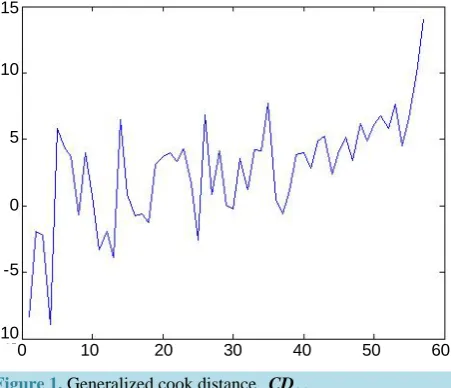
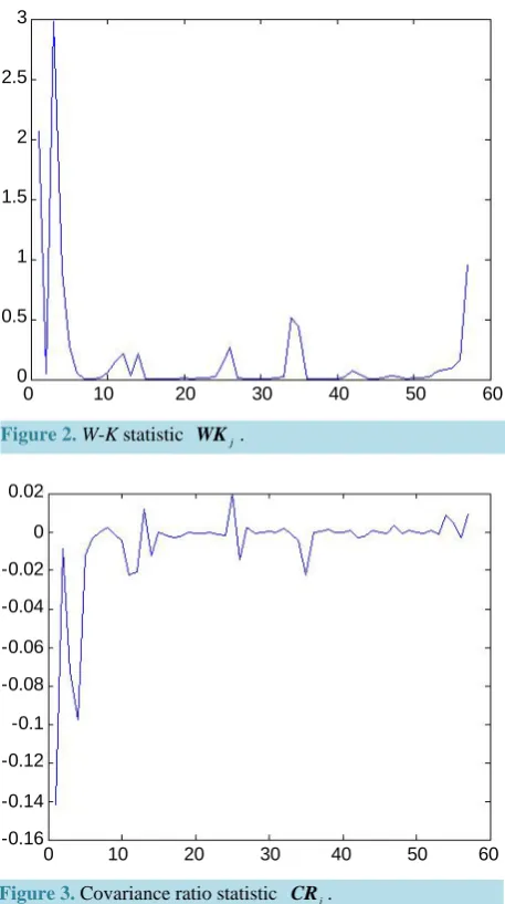
[image:6.595.202.428.521.715.2]From theFigure 1,Figure 2,Figure 3, we can see that in most cases, the value of are reasonably close to one fixed value. Following the definition and properties of diagnosis statistics, we can diagnose the strong influence points, the value of which deviate from the average seriously.Figure 2 andFigure 3 show that the first and the third data are strong influence points. Indeed, our results are illustrated.
Figure 1. Generalized cook distance CDj. 15
10
5
0
-5
-10
Figure 2.W-K statistic WKj.
Figure 3. Covariance ratio statistic CRj.
6. Conclusion
In this paper, stochastic restricted linear regression models are revisited. Useful diagnostic methods are derived. Through simulation study, we illustrate that our proposed methods can work fairly well.
References
[1] Theil, H. (1963) On the Use of Incomplete Prior Information in Regression Analysis. Journal of the American Statis-tical Association, 58, 401-414. http://dx.doi.org/10.1080/01621459.1963.10500854
[2] Hubert, M.H. and Wijekoon, P. (2006) Improvement of the Liu Estimator in Linear Regression Model. Statistical Pa-pers, 47, 471-479. http://dx.doi.org/10.1007/s00362-006-0300-4
[3] Li, Y. and Yang, H. (2010) A New Stochastic Mixed Ridge Estimator in Linear Regression Model. Statistical Papers, 51, 315-323. http://dx.doi.org/10.1007/s00362-008-0169-5
[4] Wu, J. (2014) On the Stochastic Restricted r-k Class Estimator and Stochastic Restricted r-d Class Estimator in Linear Regression Model. Journal of Applied Mathematics, 2014, Article ID: 173836.
[5] Schafrin, B. and Toutenburg, H. (1990) Weighted Mixed Regression. Zeitschrit fur Angewandte Mathematik und Me-chanik, 70, T735-T738.
[6] Li, Y. and Yang, H. (2011) A New Ridge-Type Estimator in Stochastic Restricted Linear Regression. Statistics, 45, 123-130. http://dx.doi.org/10.1080/02331880903573153
3
2.5
2
1.5
1
0.5
0
0 10 20 30 40 50 60
0.02
0
-0.02
-0.04
-0.06
-0.08
-0.1
-0.12
-0.14
-0.16
[7] Liu, C.L., Jiang, H.N., Shi, X.H. and Liu, D.L. (2014) Two Kinds of Weighted Biased Estimators in Stochastic Re-stricted Regression Model. Journal of Applied Mathematics, 2014, Article ID: 314875.
[8] He, D.J. and Wu, Y. (2014) A Stochastic Restricted Components Regression Estimator in the Linear Model. The Science World Journal, 2014, Article ID: 231506.
[9] Liu, C.L., Yang, H. and Wu, J.B. (2014) On the Weighted Mixed Almost Unbiased Ridge Estimator in Stochastic Re-stricted Linear Regression. Journal of Applied Mathematics, 2014, Article ID: 902715.
[10] Wu, J.B. and Liu, C.L. (2014) Performance of Some Stochastic Restricted Ridge Estimator in Linear Regression Model.
Journal of Applied Mathematics, 2014, Article ID: 508793.
[11] Cook, R.D. and Weisberg, S. (1982) Residuals and Influence in Regression. Chapman and Hall, New York. [12] Wei, B., Lu, G. and Shi, J. (1990) Statistical Diagnostics. Publishing House of Southeast University, Nanjing.
[13] Wang, J. (2007) Statistical Diagnosis of Linear Regression Model with the Random Constraints and BAYES Method. Nanjing University of Science and Technology, Nanjing.
[14] Yang, L. and Yang, H. (2007) Influence of Linear Model under Ellipsoidal Restriction. Chinese Journal of Engineer-ing Mathematics, 24, 60-64.
[15] Wang, L. (2008) Statistical Diagnosis of Linear Model under Linear Restriction. Nanjing University of Science and Technology, Nanjing.
[16] Durbin, J. (1953) A Note on Regression When There Is Extra Neous Information about One of the Coefficients. Jour-nal of the American Statistical Association, 48, 799-808. http://dx.doi.org/10.1080/01621459.1953.10501201
[17] Theil, H. and Goldberger, A.S. (1961) On Pure and Mixed Statistical Estimation in Economics. International Econom-ic Review, 2, 65-78. http://dx.doi.org/10.2307/2525589
[18] Özkale, M.R. (2009) A Stochastic Restricted Ridge Regression Estimator. Journal of Multivariate Analysis, 100, 1706- 1716.
[19] Hoerl, A.E. and Kennard, R.W. (1970) Ridge Regression: Biased Estimation for Nonorthogonal Problems. Technome-trics, 12, 55-67. http://dx.doi.org/10.1080/00401706.1970.10488634
[20] Hoerl, A.E. and Kennard, R.W. (1970) Ridge Regression: Applications to Nonorthogonal Problems. Technometrics, 12, 69-82. http://dx.doi.org/10.1080/00401706.1970.10488635
[21] Hoerl, A.E., Kennard, R.W. and Baldwin, K.F. (1975) Ridge Regression: Some Simulation. Communications in Statis-tics: Theory and Methods, 4, 105-123.
[22] Schaefer, R.L., Roi, L.D. and Wolfe, R.A. (1984) A Ridge Logistic Estimator. Communications in Statistics: Theory and Methods, 13, 99-113. http://dx.doi.org/10.1080/03610928408828664
[23] Kibria, B.M.G., Mansson, K. and Shukur, G. (2011) Performance of Some Logistic Ridge Regression Estimators.