Munich Personal RePEc Archive
A Latent Budget Analysis Approach to
Classification: Examples from Economics
Larrosa, Juan MC
Departamento de Economía, Universidad Nacional del Sur,
CONICET
15 September 2005
A Latent Budget Analysis Approach to Classification
Examples from Economics
Juan M.C. Larrosa1
CONICET – Universidad Nacional del Sur
Abstract
Latent budget analysis is a classification technique that allows clustering identification by using
compositional data. This paper presents examples of how this technique deals with the unit-sum constraint by establishing an initial independence model to which subsequent models are compared in terms of their relative fitness degree. In fact, latent budget analysis does not impose linearity, homogeneity, or even specific distributions on data. Results help to understand some important relationships between capital stock composition and income or food diet composition in a heterogeneous sample of countries.
FIRST DRAFT
September, 15 2005 [COMMENTS ARE WELCOME]
1. Introduction
Compositional data have restrictions for applying traditional multivariate analysis due to, among other things, the absence of an interpretable covariance structure (Aitchison, 1986). The latent budget analysis approach of compositional data is a real alternative in terms of efficiency and versatility for dealing with the analysis of this constrained data even though the sensitive advances made it from the log-ratio approach of the CODA school research contributions.
The goal of this communication is to briefly present this methodology for classification, particularly focused in economics examples. The description of the model is heavily based on van den Ark (1999) and tries to wide the knowledge of latent budget methodology for economic research application. The work follows with section 2 where the latent budget model is described, section 3 with examples from economics and section 4 ends the paper with short conclusions.
2. The Latent Budget Model
2The Latent Budget Model (LBM) is a mixture model for compositional data and enables us to obtain insights in a compositional data set without the worries of a troubled covariance matrix. By performing latent budget analysis (LBA) we approximate I observed budgets, which may represent persons, groups or objects, by a small number of latent budgets, consisting of typical characteristics of the sample. Such approximation could be used for classification, for example.
1 Contact Address: 12 de Octubre & San Juan, Planta Baja, Oficina 5, Zip Code 8000, Bahía Blanca,
The first insight into these kinds of models can be found initially in Goodman (1974a), in a more elaborated fashion in Clogg (1981) who interpreted a simple latent class model in an asymmetric way. Independently, de Leeuw & van der Heijden (1988) introduced the name ‘latent budget analysis’ because they used it to analyze time-budget data. In geological research the same model is know as endmember model (Renner 1988, 1993).
Consider and I×J compositional data matrix P, consisting of I observed budgets pi, with components pj i| .
In the LBM the observed budgets pi’s are approximated by expected budgets
π
i, which are mixtures of K(K=min
(
I J,)
) typicalcompositions or latentbudgets. The latent budgets are denoted by βk, k=(
1,K,K)
,and the model can be written as
(
)
1| 1 | | 1, ,
i i k i k K i K i I
π =α β + +K α β + +K α β = K
where αk i| 1,
(
i= K, ;I k=1,K,K)
are mixing parameters. The elements of πi and πj i| are called expectedcomponents. The elements of βk are βj k|
(
j=1,K,J)
and are called latent components. An alternativenotation for (1) is the scalar notation
(
)
| | |
1
1,..., ; 1,...,
K
j i k i j k
k
i I j J
π α β
=
= ∑ = =
and the matrix notation
T
AB
Π =
In (3) Π is a I×Jmatrix whose rows are the respected budgets; A is an I×Kmatrix of mixing parameters, and B is a J×K matrix whose columns are the latent budgets. The latent budget model with K latent budgets is denoted as LBM (K). Similar to the observed components, the parameters of the LBM are subject to the sum constraints
| | |
1 1 1
1
J K J
j i k i j k
j k j
π α β
= = = = = =
∑ ∑ ∑
and the nonnegativity constraint
| | | 0 1, 0 1, 0 1. j i k i j k π α β ≤ ≤ ≤ ≤ ≤ ≤
Thus, all the parameters are proportions and this facilitates the interpretation of the model. In fact, it has been argued that its ease of interpretation is one of the main reasons to use LBA (for example, de Leeuw and van der Heijden, 1988; de Leeuw et al., 1990; van der Ark and van der Heijden, 1998).
If the data have a product-multinomial distribution, we can compute the unconditional expected probabilities
ij
π from the expected components. The following properties hold for the expected components and the corresponding unconditional probabilities:
,
,
ij ij i
(see de Leeuw et al., 1990).
Van der Heijden, Mooijaart, and de Leeuw (1992) proposed two ways to interpret the model, which we will call the mixture model interpretation and the MIMIC-model interpretation (Multiple Indicator Multiple Cause-model). Up to now we have treated the LBM as a mixture model and the interpretation given earlier is: the LBM writes the expected budgets as a mixture of a small number of typical, or latent, budgets. Hence, each expected budget is built up out of the K latent budgets, and the mixing parameters determine to what extent. The latent budgets can be characterized by comparing them with the latent budget LBM(1). LBM(1) is the independence model, with α =1|i 1 1,
(
i= K,I)
, and βj|1= p+j(
j=1,K,J)
, in this case πi =β1 for1, ,
i= K I . Hence, if latent component βj k| is greater than that component in the independence model, p+j,
then βk is characterized by the j-th category. On the other hand, if a
β
j k| is less than p+jthen the j-th category is of lesser importance. The budget proportions πk = ∑ipi+αk i| express the relative importance ofeach latent budget, in terms of how much of the expected data they account for. At the same time,
(
)
, 1, ,
k k K
π = K denotes de probability of latent budget k when there is no information about the level of the row variable. To understand how the expected budgets are constructed from the latent budgets we must compare the mixing parameters to πk. If αk i| >πk then the expected budget πi is characterized more than
average by latent budget βk, and if αk i| <πk then the expected budget πi is characterized less than average
by latent budget βk. In practice the mixture model interpretation is carried out most easily when we first
characterize the latent budgets and then interpret the expected budgets in terms of the latent budgets.
Now, for interpreting the LBM as a MIMIC-model, we look at the observed components as conditional proportions of the row variable X, with I categories, and the column variable Y, with J categories. If we assume that the row variable and the column variable are independent given some latent variable Z with K
categories, then the LBM describes the relationship between the row variable and the column variable in an asymmetric way, i.e. π =j i| P Y( = j X| =i) denotes the probability to respond to category j of Y, given that
one belongs to the i-th category of X; these probabilities are explained by α =k i| P Z
(
=k X| =i)
which is the probability that row category i belongs to latent category k, and βj k| =P Y(
= j Z| =k)
which is theprobability that a member of latent category k responds to the j-th category of Y.
If the compositional data do not have a product multinomial distribution then the MIMIC-model interpretation may be troublesome: for example, if each observed budgets represents a multivariate observation on a single subject, then it is unclear what P Y( = j Z| =k) means. If the rows of the compositional data are not independent, for example if they denote groups, and people may belong to more than one group, then
(
|)
P Z=k Y =i is not well defined.
The parameters estimates of the LBM model should be identified before the latent budget solution can be analyzed. We follow with some examples from economics.
3. Examples from Economics
In this section we will present examples of application of LBA to economic data. We will define some economic problem to identify through LBA. When feasible, raw data will be presented and estimations will be interpreted. Following Ark (1998: 164) we will identify latent budgets by following three rules-of-thumb: a) Selecting the latent budget whose proportion of lack of fit is as large from baseline model as possible. b) The improving of adding an extra latent budget should be large enough to identify the extra effort of interpreting a larger set of parameter estimates. Ark (1998) proposes that the average improvement of fit per degree of freedom should be at least as great as the difference between the weighted Residual Sum of Squares (wRSS) of the baseline model less the observed wRSS divided by the degrees of freedom.
For a matter of exposition we are going to follow clause c with more emphasis than advisable. We follow with the first example.
3.1 Capital composition and income classification
[image:5.612.115.498.420.496.2]The first application of the latent budget analysis for a classification example is on capital composition and income. In Table 2 we see the average participation of each capital component for the 1960-1990 time periods (data were used previously in Larrosa, 2003). The definition of the components is presented in Table 1.
Table 1. Description of row variables
Code Description KDUR Percentage of capital per worker allocated in durable production assets
(machinery and equipment).
KOTHR Percentage of capital per worker allocated in other buildings.
KNRES Percentage of capital per worker allocated in non-residential building.
KRES Percentage of capital per worker allocated in residential building.
KTRAN Percentage of capital per worker allocated in transportation equipment.
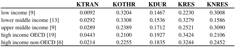
We average and closed each capital component by income category. Data are presented in Table 2 and it shed light in the long run average capital composition of the sample of countries. Notice that poorer countries possess a lower than average transportation equipment participation on capital stock and that a high-income-OECD country and a lower-middle-income country have above average residential building capital participation. Besides, poorer countries have an above from average participation of other buildings. There are 56 countries in the sample.
Table 2. Capital composition by income category (n=56)
KTRAN KOTHR KDUR KRES KNRES
low income [9] 0.0092 0.3204 0.1467 0.2230 0.3008
lower middle income [13] 0.0292 0.3308 0.1536 0.3279 0.1586
upper middle income [9] 0.0289 0.2389 0.1712 0.2521 0.3090
high income OECD [19] 0.0443 0.2100 0.1927 0.3424 0.2106
high income non-OECD [6] 0.0214 0.2255 0.1835 0.3244 0.2452
Source: column variables: Data from Penn World Table 5.6; row classification: 2000 World
Development Indicators – The World Bank. Brackets indicate the number of countries that belongs to this category.
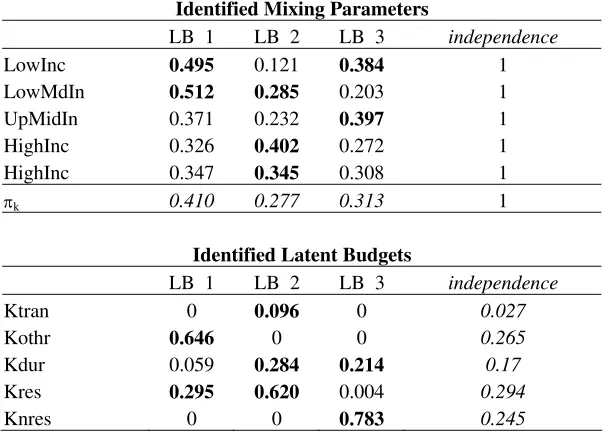
As the sample is not large and data have not additive lognormal distribution3 we could not rely on maximum likelihood estimates. We use least squares for estimating latent budgets on the model (Table 2).
3 Tests were conducted with the freeware (mvn.exe) available at http://come.to/lba/software. They are
Table 2. Estimations of mixing parameters and identified latent budgets
Identified Mixing Parameters
LB 1 LB 2 LB 3 independence
LowInc 0.495 0.121 0.384 1
LowMdIn 0.512 0.285 0.203 1
UpMidIn 0.371 0.232 0.397 1
HighInc 0.326 0.402 0.272 1
HighInc 0.347 0.345 0.308 1
πk 0.410 0.277 0.313 1
Identified Latent Budgets
LB 1 LB 2 LB 3 independence
Ktran 0 0.096 0 0.027
Kothr 0.646 0 0 0.265
Kdur 0.059 0.284 0.214 0.17
Kres 0.295 0.620 0.004 0.294
Knres 0 0 0.783 0.245
Interpretation requires going latent budget by latent budget. The first budget associates low-income countries with a higher presence of other capital al also residential capital. This would be the low-middle income budget. The second latent budget remarks the relation of residential capital and durable goods in OECD and non-OECD high income countries. This would be the high income budget. Finally, the third budget associates the non residential capital with a wider scope of countries, such middle-up and lower income countries. This would be the mid-low income budget. So far, estimations don’t shed much light into the capital composition question.
We are going to see if widening the sample helps to arrive to clearer conclusions.
3.1.1 Example 1 revisited
The former example was completed by sample averaging on World Bank’s income categories. We review the example by estimating latent variables that reveals capital composition among countries. So, this time, LBA is related to each country own data (see Table 3). This would help us to see any latent variable that conditioning capital composition in this sample. Since it would make no sense to assume a multinominal distribution and to apply a maximum likelihood estimation procedure, our weighted least squares approach seems reasonable. The weights used are 1 1 2
j
p for the columns.
Table 3. Capital composition by country (Raw data)
Country KTRAN KOTHR KDUR KRES KNRES
[image:6.612.127.486.562.726.2]FRA 0,050 0,179 0,224 0,293 0,254 GER 0,028 0,217 0,182 0,320 0,254 GRE 0,012 0,393 0,122 0,310 0,163 GUA 0,012 0,487 0,269 0,227 0,005 HKG 0,135 0,052 0,414 0,217 0,183 HON 0,174 0,194 0,417 0,122 0,091 ICE 0,018 0,071 0,112 0,613 0,185 IND 0,015 0,372 0,136 0,251 0,225 IRE 0,034 0,122 0,221 0,321 0,304 ISR 0,010 0,054 0,192 0,491 0,253 ITA 0,026 0,152 0,167 0,458 0,196 IVC 0,019 0,231 0,183 0,384 0,184 JAM 0,072 0,287 0,264 0,333 0,044 JAP 0,046 0,335 0,190 0,215 0,214 KEN 0,006 0,248 0,167 0,353 0,225 KOR 0,018 0,206 0,120 0,201 0,455 LUX 0,016 0,278 0,179 0,280 0,248 MAD 0,007 0,472 0,262 0,152 0,107 MAL 0,007 0,165 0,230 0,196 0,402 MEX 0,032 0,248 0,196 0,348 0,176 MOR 0,005 0,290 0,082 0,351 0,272 NET 0,046 0,166 0,220 0,298 0,269 NIA 0,006 0,398 0,104 0,209 0,284 NOR 0,145 0,284 0,251 0,151 0,170 NZL 0,042 0,486 0,204 0,188 0,081 OST 0,025 0,242 0,204 0,263 0,267 PAN 0,079 0,491 0,156 0,113 0,161 PAR 0,050 0,005 0,145 0,795 0,005 PER 0,011 0,387 0,112 0,485 0,005 PHI 0,005 0,044 0,148 0,220 0,584 POR 0,029 0,209 0,141 0,517 0,103 SLE 0,063 0,402 0,263 0,111 0,162 SPA 0,007 0,266 0,069 0,557 0,102 SRL 0,008 0,389 0,049 0,125 0,429 SWE 0,025 0,191 0,159 0,370 0,255 SWI 0,013 0,153 0,170 0,332 0,332 SYR 0,035 0,197 0,107 0,386 0,274 TAI 0,019 0,273 0,249 0,161 0,298 THAI 0,013 0,352 0,196 0,200 0,238 TUR 0,022 0,232 0,197 0,261 0,288 UK 0,042 0,074 0,299 0,324 0,262 USA 0,033 0,157 0,165 0,422 0,224 VEN 0,035 0,007 0,187 0,278 0,492 ZIM 0,005 0,289 0,042 0,114 0,550
Source: data processed using original data from Penn World Table 5.6
We estimate latent budgets that determine unobserved patterns in capital composition in the sample. As the sample is not large and data have not additive lognormal distribution4 we could not rely on maximum likelihood estimates. We use instead weighted least squares. First, we try to identify the model by analyzing the dissimilarity index and the mean angular deviation (van den Ark, 1999: 126-127).
Table 4. Identification of model 2
LBM(K)
Latent Budgets
1 - D m.a.d.
1/J 71.2739 0.5915
K=1 80.4209 0.3945
K=2 86.809 0.2635
K=3 90.6867 0.1955
K=4 98.4739 0.0314
As observed, as the number of latent budgets increases, the goodness-of-fit statistics (GFS) also increases. We decide for three latent budgets because of ease of interpretation and explanation of results.
Table 5. Parameter estimates of the identified mixing parameters
Country LB 1 LB 2 LB 3 Country 1 LB 2 LB 3
ARG 0.199 0.003 0.797 NOR 0.325 0.399 0.276
AUS 0.201 0.202 0.597 PAN 0.569 0.213 0.218
OST 0.282 0.141 0.577 POR 0.271 0.086 0.643
BEL 0.269 0.176 0.555 SLE 0.468 0.275 0.257
BOL 0.887 0.030 0.083 SWE 0.229 0.095 0.676
BOT 0.149 0.182 0.669 SWI 0.177 0.081 0.741
CAN 0.351 0.036 0.613 SYR 0.234 0.066 0.701
CHL 0.457 0.036 0.507 TAI 0.312 0.175 0.513
COL 0.604 0.002 0.394 THAI 0.411 0.122 0.467
DEN 0.24 0.100 0.660 TUR 0.269 0.129 0.602
DOM 0.365 0.011 0.624 UK 0.091 0.244 0.665
ECU 0.758 0.008 0.234 USA 0.194 0.111 0.694
FIN 0.266 0.092 0.642 VEN 0 0.123 0.877
FRA 0.21 0.198 0.592 GUA 0.592 0.197 0.211
GER 0.257 0.124 0.620 KEN 0.299 0.074 0.627
GRE 0.47 0.055 0.475 MAD 0.562 0.181 0.257
HON 0.227 0.596 0.176 MAL 0.179 0.128 0.693
HKG 0.061 0.511 0.428 MOR 0.342 0 0.658
ICE 0.108 0.028 0.863 NIA 0.459 0.029 0.512
IND 0.437 0.072 0.491 PAR 0.055 0.108 0.837
IRE 0.142 0.162 0.696 PER 0.487 0.042 0.472
ISR 0.078 0.087 0.835 PHI 0.022 0.04 0.939
ITA 0.194 0.1 0.705 SPA 0.336 0 0.664
IVC 0.284 0.109 0.607 SRL 0.426 0 0.574
JAM 0.356 0.281 0.362 ZIM 0.293 0 0.707
JAP 0.391 0.173 0.436 πk 0.312 0.127 0.561
KOR 0.219 0.05 0.731 Latent budgets p+j
LUX 0.327 0.105 0.568 KTRAN 0 0.252 0 0.031
MEX 0.302 0.146 0.553 KOTHR 0.845 0 0 0.264
NET 0.195 0.187 0.619 KDUR 0.045 0.727 0.12 0.174
NZL 0.578 0.19 0.232 KRES 0.111 0 0.475 0.301
KNRES 0 0.021 0.405 0.23
[image:8.612.129.490.253.603.2]Kong, Sierra Leone, Madagascar, Malawi, Taiwan and Norway, i.e., some highly developed countries are together with some of the poorest in the World.
Another way of looking at the findings is through plotting the latent budgets in ternary diagrams. Figures 1 and 2 show the same data that Table 5. Figure 1 presents latent components estimates and Figure 2 displays the calculated LBM (3). As observed, latent budget 3 (LB 3) groups most data from countries. That is, the
[image:9.612.76.536.174.352.2]building budget. At the same time, one can see that the durable goods budget is what discriminates the sample.
Figure 1. Graphic display of latent components Figure 2. Graphic display of LBM (3)
Independence model Latent budgets
LB2 LB3
LB1
LB2 LB3
LB1
3.3 Food expenditure
[image:9.612.184.428.500.710.2]Food expenditure represents the money individuals from an economy spend in feeding. This is related with socioeconomic conditions but also for cultural and religious items. We have data for the 1970 total expenditure on 32 food components from Belgium (BEL), Colombia (COL), Germany (DEU), France (FRA), U.K. (GBR), Hungary (HUN), Iran (IRN), India (IND), Italy (ITA), Japan (JAP), Kenya (KEN), South Korea (KOR), Malaysia (MYS), Netherlands (NLD), Philippines (PHI), and USA (USA). The 32 food components are detailed in Table 6.
Table 6. Food components categories
Category Labels
1 Rice 2 Flour and cereals 3 Bread
4 Other bakery products
5 Other cereal products 6 Macaroni & similar pasta
7 Beef & Veal
8 Lamb, mutton & goat meat
9 Pork meat
10 Poultry meat
11 Other fresh/frozen meat
12 Meat preparations
13 Fresh/frozen fish
14 Preserved/processed fish/seafood
16 Preserved milk/ Other milk products/ Cheese 17 Eggs
18 Butter
19 Margarine, oils & fat
20 Fresh fruit
21 Fresh vegetables
22 Dried fruit & nuts
23 Dried/frozen/prepared vegetables 24 Potatoes & other tubers/Potato products 25 Coffees
26 Teas 27 Cocoa
28 Raw & refined sugar 29 Jam/jelly/honey/s 30 Chocolate & confetti 31 Salt, spice & sauces
32 Mineral water
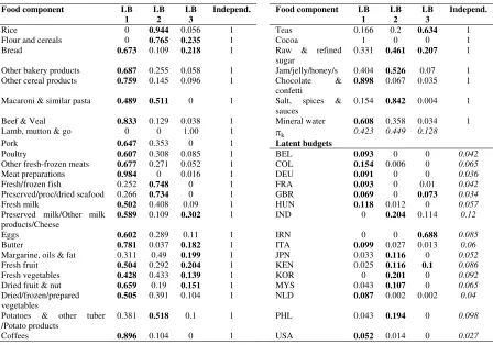
[image:10.612.84.532.380.694.2]We will try to find the latent diet of these countries by calculating the first three (unconstrained) latent budgets. Goodness-of-fit statistics show that four latent budgets could better identify the model but for ease of explanations and results visualization we stick on three. Table 7 shows the parameter estimates of the identified mixing parameters.
Table 7. Mixing parameters and latent components of the LBM (3) solution
Food component LB 1
LB 2
LB 3
Independ. Food component LB 1 LB 2 LB 3 Independ.
Rice 0 0.944 0.056 1 Teas 0.166 0.2 0.634 1 Flour and cereals 0 0.765 0.235 1 Cocoa 1 0 0 1 Bread 0.673 0.109 0.218 1 Raw & refined
sugar
0.331 0.461 0.207 1 Other bakery products 0.687 0.255 0.058 1 Jam/jelly/honey/s 0.404 0.526 0.07 1 Other cereal products 0.759 0.145 0.096 1 Chocolate &
confetti
0.898 0.067 0.035 1 Macaroni & similar pasta 0.489 0.511 0 1 Salt, spices &
sauces
0.154 0.842 0.004 1 Beef & Veal 0.833 0.129 0.038 1 Mineral water 0.608 0.358 0.034 1 Lamb, mutton & go 0 0 1.00 1 πk 0.423 0.449 0.128
Pork 0.647 0.353 0 1 Latent budgets
Poultry 0.607 0.308 0.085 1 BEL 0.093 0 0 0.042
Other fresh-frozen meats 0.677 0.271 0.052 1 COL 0.154 0.006 0 0.065
Meat preparations 0.984 0 0.016 1 DEU 0.091 0 0 0.036
Fresh/frozen fish 0.252 0.748 0 1 FRA 0.093 0 0.01 0.042
Preserved/proc/dried seafood 0.266 0.734 0 1 GBR 0.069 0 0.073 0.034
Fresh milk 0.502 0.408 0.09 1 HUN 0.118 0.012 0 0.057
Preserved milk/Other milk products/Cheese
0.589 0.109 0.302 1 IND 0 0.204 0.114 0.12
Eggs 0.602 0.289 0.11 1 IRN 0 0 0.688 0.085
Butter 0.781 0.037 0.182 1 ITA 0.099 0.027 0.013 0.06
Margarine, oils & fat 0.311 0.49 0.199 1 JPN 0.033 0.116 0 0.052
Fresh fruit 0.504 0.292 0.204 1 KEN 0.025 0.116 0.1 0.086
Fresh vegetables 0.428 0.433 0.139 1 KOR 0 0.201 0 0.092
Dried fruit & nut 0.659 0.19 0.151 1 MYS 0.043 0.107 0 0.065
Dried/frozen/prepared vegetables
0.505 0.391 0.104 1 NLD 0.087 0.002 0.002 0.04
Potatoes & other tuber /Potato products
0.381 0.518 0.1 1 PHL 0.043 0.194 0 0.098
Interestingly, interpretation begins with latent budget one that represents all Western countries in the sample. This would be the Western diet budget. Related to this culture pattern we could match a basket of food items as represented by the mixing parameters relatively to the budgets proportions: So, Western diet budget includes meat preparations, coffee, beef and veal, chocolates, cereals, butter, other fresh meats, mineral water and other food components. The second latent budget reflects a higher value for countries other than Western. The majority are Asian countries, so this would be the Asian diet budget. This basket reflects higher than average presence of rice, salt and spices, fresh and processed fish, flour and cereals, potatoes, jams and jellies, pastas and sugar. Finally, the third latent budget is highly represented by a Muslim country like Iran, with low participation of other Western and African countries. The most important food component is tea. So, this would be the tea diet budget5 and indicates a higher presence of, of course, tea, cheese and preserved milk, fresh fruits, floor and cereals, bread, margarine and oils and other foods components. Would you expect a clearer picture?
We end this communication with the conclusions.
4. Conclusions
Latent budget analysis is an attractive alternative for dealing with compositional data. As reported, it is easy to use and to interpret the results. It deals with highly problematic and widely available data. This report, inconclusive and still incomplete, tries to be an introduction for more insightful and in-depth texts, as van den Ark (1999) is.
As described above, LBA seems to be ideal for statistical classification and searching for unobserved patterns in data. These kinds of problem are a common in social sciences. We hope this tool rapidly enters in the syllabus of standard grade statistics course.
Acknowledgments
LB estimations were made using the freeware (lba.exe), by van den Ark, Mooijart and Van der Heijden at http://come.to/lba/software. Ternary diagrams were made it with the freeware Codapack (see Thió-Henestrosa and Martín-Fernández, 2005).
References
Aitchison, J. (1986). The Statistical Analysis of Compositional Data. London, New York: Chapman and Hall. 417 p.
Ark, Van der L.A. (1999). Contributions to Latent Budget Analysis; A Tool for the Analysis of Compositional Data. Leiden: DSWO-press.
Ark, Van der L.A., and P.G.M. Van der Heijden (1996). Geometry and Identifiability in the Latent Budget Model. (Methods Series MS-96-3). Utrecht: Utrecht University, Faculty of Social Sciences, ISOR. Ark, Van der L.A., and P.G.M. Van der Heijden (1996). “Graphical Display of Latent Budget Analysis and
Latent Class Analysis, with Special Reference to Correspondence Analysis”. (Methods Series MS-96-4). Utrecht: Utrecht University, Faculty of Social Sciences, ISOR.
Ark, Van der L.A., and Van der Heijden, P.G.M. (1998). “Graphical display of latent budget analysis and latent class analysis, with special reference to correspondence analysis”. In J. Blasius, & M. Greenacre (Eds.), Visualization of Categorical Data, (pp.489-509). San Diego: Academic Press. Ark, Van der L.A., P.G.M. van der Heijden, and D. Sikkel (1999). “On the identifiability in the latent budget
model”. Journal of Classification16: 117-137.
Clogg, C.C. (1981). “Latent structure models of mobility”. American Journal of Sociology86: 836-868. de Leeuw, J., and P.G.M. Van der Heijden (1988). “The analysis of time-budgets with a latent time-budget
model”. In E. Diday (Ed.) Data Analysis and Informatics V: 159-166. Amsterdam: North-Holland.
de Leeuw, J., P.G.M. Van der Heijden and P. Verboon (1990). “A latent time budget model”. Statistica Neerlandica44: 1-21.
Heijden, Van der P.G.M. (1994). “End-member analysis and latent budget analysis”. Applied Statistics,
Journal of the Royal Statistical Society, Series C, 43: 527-530.
Heijden, Van der P.G.M., A. Mooijaart, and de Leeuw, J. (1989). Latent budget analysis. In A. Decarli, B.J. Francis, R. Gilchrist, and G.U.H. Seeber (Eds.). Statistical Modelling. Proceedings of GLIM 89 and the 4-th International Workshop on Statistical Modelling, Lecture Notes in Statistics 57: 301-313. Berlin: Springer-Verlag.
Heijden, Van der P.G.M., L.A. Van der Ark, and A. Mooijaart (1999). “Some examples of latent budget analysis and its extensions”. In A.L. McCutcheon, and J.A.P. Hagenaars (eds.). Advances in Latent Class Modeling Cambridge: Cambridge University Press.
Larrosa, J.M.C. (2003). “A compositional statistical analysis of capital stock”. Documento de Trabajo 5, Instituto de Economía, Universidad Nacional del Sur.
Mooijaart, A., P.G.M. Van der Heijden, and L.A. Van der Ark (1999). “A least squares algorithm for a mixture model for compositional data”. Computational Statistics and Data Analysis30: 359-379. Thió-Henestrosa, S. and J.A. Martín-Fernández (2005). “Dealing with compositional data: the freeware