Current Trends in Parallel Computing

Current Trends in Parallel Computing

Rafiqul Zaman Khan

Aligarh Muslim University Aligarh, UP, INDIA.

Md Firoj Ali

Department of Computer Science Aligarh Muslim University

Aligarh, UP, INDIA

ABSTRACT

In this paper a survey on current trends in parallel computing has been studied that depicts all the aspects of parallel computing system. A large computational problem that can not be solved by a single CPU can be divided into a chunk of small enough subtasks which are processed simultaneously by a parallel computer. The parallel computer consists of parallel computing hardware, parallel computing model, software support for parallel programming. Parallel performance measurement parameters and parallel benchmarks are used to measure the performance of a parallel computing system. The hardware and the software are specially designed for parallel algorithm and programming. This paper explores all the aspects of parallel computing and its usefulness.

Keywords

Parallel computing, parallel computing hardware, parallel model, parallel benchmarks.

1. INTRODUCTION

A processor has its own physical limits in maximum processing speed. To overcome this limitation multiple processors are connected co-operating with each other to solve grand challenge problems. The parallel computing refers to the processing of multiple jobs simultaneously on multiple processors. A large problem can be divided into multiple independent tasks of nearly same size by applying an appropriate task partitioning technique and each of the tasks will be executed on different processors simultaneously. Numerous application problems today needs more and more computing power than a usual sequential computer. A large problem either may take long time or indefinite time to finish when it is processed on a single processor. The time taken to finish the problem may be too much to have any importance or it may be obsolete for real time computing. So the clear solution of the above problem is the parallel computing that ensures a cost-effective solution by connecting more number of processors through the high speed communication mediums. Parallel computing model is mainly of two types. First one is shared memory and second one is distributed computing. In shared memory architecture a number of processors are connected to a common shared memory. Data or instructions are shared through locks and semaphores. It is easy to program but sometimes mislead the results. In distributed computing the independent processors having their own memory are connected through a fast communication medium. Data and information are shared through message passing. It is difficult to implement but yields better computing performance. There is another model known as hybrid model which imbibes both the concepts from shared memory model and distributed model.

Assigning the tasks to the processors is not just the solution of the problem in parallel. Some faster processor may sit idle while a slower processor may busy in a parallel computing system resulting slower computing speed due to the uneven distribution of tasks. The number of tasks on a processor is

called work load. Some processors may have more work load than others and hence some processors may be overloaded and lightly loaded causing an imbalance in task idle time. For an efficient parallel computing system the task idle time will be as small as possible. The work load from the overloaded processors can be shared by the lightly loaded processors by invoking an appropriate balancing algorithm. The workload should be equally shared when the computing system is homogenous otherwise faster processors should process more numbers of jobs than slower processors per unit time to keep better performance of the system.

2. PARALLEL COMPUTING

HARDWARE ARCHITECTURE

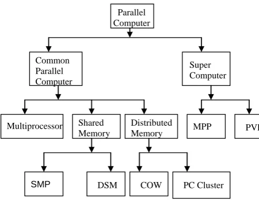
A revolutionary change has been done in the last decade in hardware development related to the computation. There exist several parallel computing hardware architectures. Depending upon the cost and the type of computational problem parallel computing hardware architecture can be divided mainly into two categories: common parallel computer architecture and super computer architecture. A classification of parallel computer is shown in Fig 1. Super computers are very expensive and take long time to produce. Each parallel application does not need dedicated super computer and most of the organizations can not buy a super computer due to its high cost. Fortunately a new alternative concept has emerged that is known as common parallel computing in which a large number of systems which consists of cheap and easily available autonomous processor like workstations or PCs. So it is becoming extremely popular for large computing purpose such as scientific calculations as compared to super computers.

2.1. Common Parallel Computing

Architecture

In this architecture non-dedicated computers which are easily available are connected through a high speed communication media to act as a parallel computer. The architecture requires very less effort and can be built with negligible cost if the general purpose computers are available. The combined processing power and the storage capacity solve many big problems in parallel easily those were not possible to solve otherwise. Common parallel computers have been divided into three categories: multiprocessor computer, shared memory and distributed memory computing architecture.

In multiprocessor architecture more than one CPU is incorporated to a single computer. The compiler is responsible for parallelizing the code automatically. This type of architecture is not so efficient but better than a computer with single CPU.

Since all processors are sharing a single address space, the data sharing is fast but processes can corrupt each others data at the same time. So the semaphores and locks are used to save the data from corruption. There is a lack of scalability between PEs and memory which means that we can not add PEs as many as we need to a limited memory. This problem arises mainly due to the bus contention [12, 16]. The examples of SMP machines are IBM R50 SGI Power Challenge, DEC Alpha Server 8400. Distributed shared memory (DSM) is another type of shared memory architecture. In DSM memory is dedicated to each processor but the memories are connected through a bus to form a shared memory and the inter process communication takes place through shared variables. Although the memory is distributed in DSM, the system hardware and software make it as single address architecture. DSM removes the problem of bus contention and provides better performance than SMP. DSM architecture machines are Stanford DASH, SGI Origin 2000 and Cray T3D.

In distributed shared memory all the PEs which are connected through a network have their own independent local memory in distributed memory MIMD computer. Each PE is a full computer connected through a network. This architecture is also known as loosely coupled because the PEs are not tightly integrated as in shared memory architecture. As a PE can not directly access the memory of other PEs, it is called No Remote Memory Access (NORMA). PEs can communicate with the others through the communication network by message passing. The network that connects the PEs may be of different topologies like bus, tree, mesh, cube etc. Cluster of workstation (COW) and PC cluster fall under this category [7, 9, 14]. A cluster is a collection of independent computers that are physically interconnected through LAN with the high performance network technology like FDDI, Fiber Channel, ATM switch etc.

2.2. Super Computing Architecture

Super computing has extremely high execution rate and extremely high I/O throughput. It needs very large primary and secondary memory. So the cost and the time are the two crucial factors for producing super computers. The principal architectures of super computing are Massively Parallel Processor (MPP) and Parallel Vector Processor (PVP) [9, 14]. MPP system is the collection of hundred or thousand of commodity processors interconnected by high speed and low latency communication network. The memory of the processors in MPP is distributed but the processors are synchronized by the blocking message passing operations. Each process has its own physical address space and communicates with the others through message passing primitives. Intel paragon, Cray T3E and TFLP are the examples of this category. PVP uses specially designed few vector processor of capacity having at least 1 Gflop/s performance thus PVP can maintains an extremely well performance for some particular applications and naturally they are expensive than MPP. PVP makes the use of huge number of vector registers and instruction buffer instead of cache. Cray C-90, Cray T-90 and NEC SX-4 are the example of PVP machines. A list of top ten supercomputers [13] has been shown in TABLE 1.

3. PARALLEL COMPUTING MODEL

The need of parallel computing model arises to solve any problem in order to facilitate analysis and prediction. The models are used for developing efficient problem solving tools and thus a model is utilized to solve a particular class of a problem. A good computational model can make any complicated problem easier to the program designer and

developer. It also simplifies the way of mapping load effectively onto real computers.Different parallel computing models are used to solve parallel problems. According to the memory model the parallel computational model can be divided into three categories: shared memory computational model, distributed computational model and hierarchical memory model. We introduce the above models in brief.

3.1. Shared Memory Parallel Computing

Models

In shared memory architecture a number of processors are connected to a common central memory. Since all processors are sharing a single address space, the data sharing is fast but processes can corrupt each others data at the same time. So the semaphores and locks are used to save the data from corruption. There is a lack of scalability between PEs and memory which means that we can not add PEs as many as we need to a limited memory.

3.1.1. PRAM Model

PRAM model is relatively older and widely used shared memory computing model for the design and analysis of parallel algorithms and was first developed by Fortune, Wyllie and Goldschlager. A limited numbers of processors share a common global pool of memory. The processors can operate synchronously and allowed to access the memory concurrently and take only one unit of time to be completed. Imposing the restrictions on memory access, the PRAM model has different instances. CRCW PRAM model [15] that permits simultaneous read and write to the same memory cell. CREW PRAM [15] is another model that permits simultaneous read to the same memory cell but permits only one processor to write on a cell at a time. Another model which does not permit the concurrent access of any given memory cell is known as EREW PRAM. Another model which uses limited communication bandwidth by calculating maximum memory contention in each phase of algorithm is known as QSM model. Though the PRAM model is easy to implement, it suffers from memory and network contention problem.

3.2. Distributed Memory Parallel Computing

Models

There are numbers of distributed memory parallel computing models in which each complete computer having their own memory are connected through a communication network. Model BSP and LogP models are the most well known models under these Models. These models remove the shortcomings of the shared memory computational memory. We introduce both of them in brief.

3.2.1. BSP Model

3.2.2. LogP Model

LogP model consists of four parameters- P numbers of computers, L (latency of message passing), O (overheads involved in message passing) and g (minimum time interval between successive messages) [8]. At most L/g messages can be transmitted from one processor to another at any instant. If a process has more than this number of messages to transmit, it stalls until the message can be sent without exceeding the capacity limit. This model is asynchronous in nature and thus message passing latency is unpredictable. In this model all this parameters are not considered at the same time, some of them can be neglected For example, some algorithms that does not communicate data frequently, the bandwidth and capacity limit can be ignored.

3.3. Hierarchical Memory Computational

Models

The speed of processor is more and more than the speed of memory. So the cost of memory access should be considered. Since the access time of different memory location is different, a more precise communication cost can be evaluated and the performance of the model can be predicted more efficiently. This model is very suitable when the bulk of data movement among different level of memory hierarchy occurs for some class of problems.

Hierarchical memory model (HMM) [1] and hierarchical memory model with block transfer (HMM with BT) [2] are the two early models of parallel computational model with memory hierarchy. In HMM model, there are K levels of memory each of which contains 2K memory locations; access to memory location x takes f(x) time for some function f. HMM with BT model is slightly different from HMM in the sense that HMM with BT model transfer data in large block ended at address a with length l will have cost f(a) + l.

3.3.1. UMH Model

This model is different from the above models. The cost function for the memory access is the function of memory level numbers not data addresses. Another difference is that UMH model allows the simultaneous data transfer on different level buses while HMM and HMM with BT only allow one transfer at a time.

3.3.2. HPM Model

HPM is a memory hierarchical model for general homogeneous parallel computer systems with hierarchical parallelism and hierarchical memories. It contains hierarchy of enhanced RAMS that co-operate with each other. In HPM model, the level K is used for memory access and level K+ is used for message passing. Its organization of hierarchical memories has many common features as UMS and DRAM models.

4. PARALLEL PROGRAMMING DESIGN

and IMPLEMENTATION

There are three main approaches for designing the parallel algorithm. First one is the parallelization of a sequential problem which has the chance of parallelism inside it. The inside parallelism can be exploited to make it parallel. The second one is the way of parallelization of any new problem at the start time. The third one is that taking any well known algorithm and solves the problem accordingly.

There are several ways of designing a parallel algorithm. The most widely used techniques are portioning, divide and conquer, pipelining etc. in partitioning, a problem is divided

into sub-problems of nearly equal size which will be non-overlapping. The sub-problems will be then solved concurrently. In divide and conquer the problem will be broken first into sub-problems. The sub-problem will be solved recursively and the result of the sub-problems merged at the end. Pipelining is the simple but good technique for parallel algorithm. The problem will be divided into segments and the output of one segment is the input of another next segment and they produce the result at the same rate.

Decomposition, assigning, mapping and scheduling are the common way to implement the parallel algorithm. A proper division of a large problem into a number of sub-problems can facilitate the effective implementation of a parallel algorithm. There are two main techniques for the decomposition of a problem. First one is domain decomposition and second one is functional decomposition.

In domain decomposition the data associated with the problem is divided into small pieces of data of nearly equal in size. Now the algorithm is divided in such a way that to operate on each task. Different tasks are given to operate on different data. In domain decomposition tasks start simultaneously.

Functional decomposition divides the algorithm into independent tasks which can be processed simultaneously. If the data needed for the tasks is also independent, the division is perfect otherwise the communication will be considerable to avoid the repetitions of data. All tasks commence concurrently but some of the tasks will have to wait until data is obtainable.

5. SOFTWARE SUPPORT for

PARALLEL PROGRAMMING

Designing a parallel programming is always challenging matter. More and more focus is imposed on designing parallel programming design. Two methodologies are widely used for the purpose of parallel programs. They are auto-parallelization compiler and library based software.

Auto parallelization does its work in two fashions. First one is complete automatic compiler which finds the parallelism during the compilation of source code. This approach mainly aims to

parallelize the loops like for and do. Second one is program directed which uses compiler directives to make the code parallel.

The library based parallel software embedded its library to the sequential programming languages to support the parallel execution of a problem. MPI and OpenMP are the most widely acceptable standard for parallel programming. MPI is a common message passing library which has the primitive function like send() /receive() by which MPI process communicate with the other process through message passing. OpenMP is a parallel framework for supporting compiler directives, library support routine. Apart form this LINDA, CPS, P4 etc are the example of parallel programming software.

6. PARALLEL PERFORMANCE

MEASUREMENT

We will introduce some performance measurement parameters- execution time, speedup, efficiency and scalability. Each parameter has its own way of describing the characteristics of the parallel program.

6.1. Execution Time

minimum that is lower the value of execution time better is the performance of a system. Generally execution time is denoted by Ts and Tp where Ts represents the execution time for a fastest sequential problem and Tp represents the execution time for a parallel problem on p processors. There is a relation between Ts and Tp that will found in other parameters below.

6.2. Speed-up

Speed-up measures how many times a parallel program works faster than a sequential one when both programs solve the same problem. Speed-up is denoted by Sp which is the ratio of Ts and Tp and can be represented as

Tp

Ts



Sp

Hence Sp measures the benefit of parallel computer over sequential computer. The highest value of Sp can be equal to the number processors used in parallel computer when there will be no communication among the processors which is impractical situation in parallel computing. So due the communication cost the speed-up is always less than equal the number of processors used in parallel computer.

According to the Amdahl’s law [3], it is very difficult to get ideal parallel system to get the value of Sp is equal to p due to the presence of some sequential code which can not be parallelized and must be processed sequentially by a single processor. Suppose r is the part of a program that can be parallelized and the rest s = 1-r part is sequential in nature. Then the speed up becomes

p

r

s

Sp

/

1





When p





s

1



speed-up can be achieved is less than equal to 1/s whatever may be the number of processors present in the system.

6.3. Efficiency

Efficiency measures the number of operations performed by the processors during the parallel execution. The efficiency can be formulated as





100

p

Sp

Ep

Where Sp is speed-up and p is the number of processors used in parallel system. Ep represents the contribution of the processors to the parallel execution.

7. PARALLEL BENCHMARKS USED in

HPCC

Another way of measuring the performance of a parallel system is done by applying parallel benchmarks. Benchmarks are freely available standardized computer programs that are mostly used by the HPC community to measure the system performance. The new benchmarks are being created for making it standardized so that every industry, manufacturer and customer can use the benchmarks to evaluate the performance of a computer system. There are mainly three types of benchmarks: synthetic benchmarks, kernel benchmarks and real application benchmarks. Synthetic benchmarks are small programs and it does not perform any real computation but work out the basic

functions of a machine. It compares the relative efficiency of processors. Example of this category is Whetstone benchmark, Dhrystone and wPrime etc. In Kernel benchmarks a part of a large program is extracted and this part of program is responsible for most of the execution time of that problem. Examples are LINPACK, NAS etc. In real application benchmarks the code segment is the application program itself. It is very effective in measuring the overall system performance but needs more time resources. Examples are Perfect Benchmarks, SPEC benchmarks etc. we represent some of the benchmarks which are mostly used to evaluate the performance.

7.1. Whetstone Benchmarks

Whetstone benchmark was the first international benchmark in history [10]. It was intended to measure the performance of a computer system and to simulate the floating point intensive application problems. It consists of nine small loops of different statement of particular type like integer arithmetic, floating point arithmetic, ‘if’ statements etc. It uses global variables and a high percentage of execution time is spent in mathematical library functions. The result of this benchmark is represented in MWIPS (mega whetstone institution Per Second).

7.2. Dhrystone Benchmarks

It was built to measure the performance of non numeric applications. It consists of measurement loops. Each loop includes twelve procedures and ninety four statements. One hundred one statements are dynamically executed during one Dhrystone [18]. Dhrystone benchmarks do not contain any floating point operations and most of its operations involve string operations. These benchmarks are widely acceptable by the business vendors because the working set of the program fits properly in the cache of modern computer machines.

7.3. LINPACK

These benchmarks are used to measure the performance of a computer system when a dense system of linear equations is solved by applying Gaussian elimination method [11]. The benchmarks are involved in calculating high percentage of floating point calculation in double precision. Most of the execution takes place just 15-line subroutine of the program. The result of these benchmarks is expressed in MFLOPS. These benchmarks are widely used by TOP500 and China TOP100 [7].

7.4. NAS Kernel

NAS consists of seven kernels which has the size of 1000 lines in total. These are developed by the NASA Ames Research Center. Each kernel is independent to each other and does not depend on the result of other kernel. Each kernel has a loop that iteratively calls a particular subroutine [4]. The performance of these benchmarks is expressed in MFLOPS.

7.5. Perfect Benchmarks

7.6. HPCC Benchmarks

HPCC benchmarks consist of seven computational kernels: STREAM, HPL, DGMM, PTRANS, FFT, RandomAccess and b_eff. HPCC benchmarks are applied to measure performance from single computer to largest supercomputer. HPCC Benchmarks measures processor’s memory bandwidth, memory speed, random updates of memory, transfer of data, latency and bandwidth of communication. The summary of the above benchmarks are shown in TABLE II.

8. CONCLUSION

In this paper all the necessary aspects of parallel computing has been represented. Hardware architecture for parallel computing as supercomputing architecture and common parallel computing architecture are discussed. We also discussed about Shared and Distributed memory models. We also observed that Shared memory model is faster but suffers from memory contention which is overcome by the Distributed memory model. Parallel computing needs the special software for performing the parallel processing. MPI, OpenMp and PVM etc are the parallel software library for executing any parallel application. Some popular parallel bench marks are briefly discussed in this paper for measuring the performance of different types of parallel problems. Each benchmark is specific to each type of problem and thus a suitable benchmark would be chosen from Table 2 depending on the nature of the problem.

Fig.1: A Classification of Parallel Computer

Table 2. Summery of the above benchmarks

S.N o

Benchmar k

Benchmark Type

Application Type 1 Whetstone Synthetic Floating point

intensive application problems 2 Dhrystone Synthetic Non numeric

applications 3 LINPACK Kernel Dense system

of linear equations 4 NAS Kernel Kernel Numerical

Aerodynamic Simulation 5 Perfect Application Measures

performance of super computer

6 HPCC Extend

version of LINPACK

Measures performance from single computer to largest supercomputer

Parallel Computer

Common Parallel Computer

Super Computer

Multiprocessor Shared Memory

Distributed Memory

SMP DSM COW PC Cluster

Table1. Top ten supercomputer of the world 2.34 1.042 122400 USA Roadrunner

BladeCenter QS 22/LS 21 IBM DOE/NNSA/LANL 10 4.59 1.050 138368 France Tera 100

Bull bullx super-node S6010/S6030 Bull Commissariata 1’Energie Atomique (CEA) 9 2.91 1.054 153408 USA Hopper

Cray XE 6, 6C 2.1GHz Cray DOE/SC/LBNL/ NERSC 8 4.10 1.088 111104 USA

Pleiades SGI Altix ICE 8200EX/8400EX SGI NASA/ Ames Research Center/NAS 7 3.98 1.110 142272 USA

Cielo Cray XE6, 8C 2.4 GHz Cray DOE/NNSA/LANL/ SNL 6 1.40 1.192 73278 Japan

TS UB AME-2

HP ProLiant, Xenon 6C, NVidia, Linux/ Windows

NEC/ HP GS IC, Tokyo

Institute of Technology 5 2.58 1.271 120640 China

Nebulae TC 3600 Blade, Intel X5650, NVidia Tesla C2050 GPU Dawning National Supercomputing center Shenzhen 4 6.95 1.759 224162 USA

Jaguar Cray Xt5, HC 2.6 GHz Cray

Oak Ridge National Laboratory 3 4.04 2.566 186368 China Tianhe-1 A NUDT TH MPP NUDT

National Supercomputing center in Tianjin 2 12.66 10.51 795024 Japan K Computer

SPARC64 VIIIfx 2.0 GHz, Tofu Interconnect Fujitsu Riken Advanced Institute for Computational Science 1 Power (MW) R max (PFlops) cores Country Computer Manufacturer Site Rank

9. REFERENCES

[1] Aggarwal A., Alpern B., Chandra A. and Snir M. “A Model for Hierarchical Memory”. Proc of 19th

Annual ACM Symp. on Theory of Computing, ACM, pp. 305-314, May 1987.

[2] Aggarwal A., Alpern B., Chandra A. and Snir M. “Hierarchical Memory with Block Transfer”. Proc of 28th Annual IEEE Symp. on Foundations of Computer Science, pp. 204-216, 1987.

[3] Amdahl G. M. “Validity of the Single-processor Approach to Achieving Large Scale Computing Capabilities”. In AFIPS Conference Proc., Atlantic City, New Jersey, pp.483-485, 1967.

[4] Baily D.H and Barton J.T. “The NAS Kernel Benchmark Program”. Tech. Rep., Numerical Aerodynamic Simulation (NAS) System Division, NASA Ames Research Center, June, 1986.

[5] Berry M, chen D, Koss P, Kuch D, Lo S and Pang Y. “The PERFECT Club Benchmarks: Effective Performance Evaluation of Super Computers”. Tech. Rep., PERFECT Club, July, 1994.

[6] Chen G, Sun G, Zhang y and mo Z. “Study on Parallel Computing”. Journal of Computer Science and Technology, vol. 201, no. 5, pp. 665-673, Sept. 2006.

[7] Chen G. and An H. et al. “Parallel Algorithm Practice ”. Higher Education Press, 2003.

[8] Culler D, Karp R, Patterson d et al. “LogP: Towards a Realistic Model of Parallel Computation”. In Proc. ASPLOS IV, Nw York, 1993, pp. 1-12.

[9] Culler D.E. et al. “Parallel Computer architecture”. Morgan kaufman Publishers, 1999.

[10] Curnow H.J and Wichman B.A. “A Synthetic Benchmark”. Computer Journal, vol19, no. 1, Feb 1976.

[11] Dongrra J.J. “Performance of Various Computers Using Standard Linear Equation Software”. Tech. Rep. CS-89-85, University of Tennessee and Oak Ridge National Laboratory, November, 1995. [12] Flynn M. J. “Computer Architecture: Pipelined and

[14] Hwang k. et al. “Scalable Parallel Computing”. McGraw-Hill, 1998.

[15] Jaja J. “An Introduction to Parallel Algorithms”. Addison-Wesley, 1992.

[16] Protic J. et al. “Distributed Shared Memory: Concept and Systems”. IEEE Parallel and Distributed Technology, Summer 1996.

[17] Valiant L. “A bridging Model for Parallel Computation”. Communication of ACM, 1990, 33: 103-111.