The Multi-Agent System and Stochastic Process in the
Road Traffic
Gouiouez Mounir
Laboratory Computer and
Modeling, University, Fez,
Morocco
N. Rais
Laboratory Computer and
Modeling, University, Fez,
Morocco
M. Azzouzi Idrissi
Laboratory Computer and
Modeling, University, Fez,
Morocco
ABSTRACT
In recent years, the rapid growth of road traffic density generates a rising request for tools that can be used to analyze and control the traffic networks. The Microscopic traffic simulation is one of the major tools used in the analysis of traffic systems; it provides a very detailed study of the interaction between the elements of the traffic network. Thus microscopic traffic simulation has become an ever increasing field of research and development.
The main aim if this paper is to provide a new model for microscopic traffic simulation; Traditional traffic simulation models neglect some real-life factors that need to be considered, such as the effect of random distribution in the entry of lane. This paper combines the Multi-Agent Systems (MAS) and the stochastic process to model the randomness of vehicles arrival at the entry of the lane.
The second contribution of this paper is about the internal structure of mobile agents[8] which initially reacts according to the instructions of the Main agent (MA); in the case of a lack of dynamic information, the mobile agents take decisions based on their experiences accumulated during previous interactions. The obtained results illustrate that using the randomness in the reaction of agent enhanced greatly the performance of simulation.
Keywords
Multi-Agent system, Microscopic Traffic Simulation, Random Distribution, Poission Law
1. INTRODUCTION
The theoretical characteristics of the simulation of traffic systems and mathematical analysis must be applied and evaluated in accordance to reality. The process of evaluation will determine the effectiveness of the provided model. Hence, the combination between the mathematical analysis and Microscopic Traffic Simulation has proven to be one of the most useful tools for analysis of various traffic systems. The microscopic simulation focuses on the study of each component of the traffic system individually; every individual vehicle is modeled as a single simulation object. These simulated vehicles drive along the streets, change traffic lanes and their driving directions as they interact with each other. Each simulated vehicle has its own immediate position, speed, and acceleration in the traffic flow …etc. The most important models in this area are the car following model [9] and cellular automaton model [10].
In the mathematical analysis, Traffic flow has been considered as a stochastic process. (Adams 1936)[22] proposed the idea of vehicles arrival at the entry of lane as a random process and verified its relevance to theory and observations. Afterwards, (Greenberg 1966)[23] has found a connection between the microscopic traffic flow theory and the lognormal follower headway distribution. In 1993 Heidemann[24] developed a new approach in which he applied the theory of stochastic processes to analytically derive the headway distribution as a function of traffic density. His approach may provide a link between the macroscopic traffic flow theory and the headway distributions. Multi-Agent System has brought a new vision to study the microscopic phenomena and complex situations with emphasizes the interactions of components of the systems. In literature, the MAS is one of the newest area of research in the artificial intelligence (AI), it has started in the early 90s with (Minsky 94)[25], (Ferber 95)[26], as an attempt to enrich the limits of classical AI[11]. The foundations of the MAS are interested in modeling human behaviors in the real world with mental notions such as knowledge, beliefs, intentions, desires, choices, commitments (Shoham, 1993)[27].
There are various definitions of the concept agent [12, 13, 14] in the contemporary literature; however, the adopted definition which covers the characteristics of agents developed in the new model, is that proposed by Jennings, Sycara and Wooldridge (JEN 98)[28]:
For Jennings, Sycara and Wooldridge an agent is a computer system, located in an environment, which is autonomous and flexible to meet the objectives for which it was designed. As far as MAS is concerned, according to Ferber (Ferber 95)[30] a MAS is a system composed of the following: Environment, a set of objects in space; a set of agents who are active entities of the system; a set of relationships that binds objects together; a set of operations allowing agents to perceive, destroy, create, transform, and manipulate objects.
Therefore, the main objective of the research is to develop a new microscopic approach in the MAS combining the notion of theoretical mathematic model, especially the statistic model, and the main characteristics of the Multi-agent System. Such a combination would pave the way for a real description of the phenomena.
simulation. The structure of this paper is divided into five sections; the first section provides a general overview microscopic simulation. The second section describes the new architecture. Section three presents the combination of the new model and AIMSUN2 Simulation Process. The experimental results are presented and discussed in Section four. Finally, Section five concludes the paper.
2.
MULTI-AGENT
ARCHITECTURE
DESCRIPTION
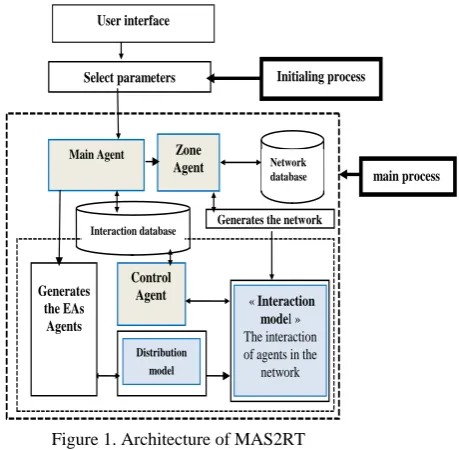
In traffic simulation two processes can be distinguished. First of all, the initialing process is composed of modules responsible of starting the simulation. The second process or the main process is, in the case of proposed architecture, comprised of multiple interacting intelligent agents.
The main process consists of a distribution model which is used to define the affectation method in the network. The interaction model is used to regulate the interactions between the agents. In design of this architecture, the aim was to explicitly build a distributed and decentralized solution, where each agent performs its own task. The resulting architecture will then capitalize on effective use of distribution to avoid bottlenecks and achieve scalability with an increase in a number of transactions.
The architecture is schematically depicted in Fig. 1 which shows the architectural components. The Main Agent (MA), which is the main element of this architecture, serves to distribute the Execution Agents (EAs) – vehicles - in the network following the distribution model and supports these agents to locate all required resources designed by Zone Agent (ZA). This latter present the ground in which the (EAs) interact among each other according to the interaction model.
ZA is the agent responsible of building network from a database that contains all the elements necessary to build a network (roads, crossroads ...). Besides, during the simulation, it provides all information about the positions of EAs to the Control Agent (CA).
CA is designed to build a re-active and persistent architecture. This agent records the evolution of architecture caused by changes of existing resources in the interaction database which discern the change in the behaviors of the EAs.
In the proposed approach, CA collect all information of the execution agents Thus, the accumulated information could be shared between agents, increasing overall efficiency of the system. During registration, the MA aims to retrieve EAs’ characteristics in the interaction database; hence, EAs update their knowledge about the other agents. This process of update is decided according to the collected information by the CA.
User interface
Control Agent
Main Agent
Generates the network
Distribution model
« Interaction model » The interaction of agents in the network Generates
the EAs Agents
Select parameters
Zone Agent
Initialing process
main process Network
database
Interaction database
Figure 1 sheds light on the links between all agents and models of the architecture. In order to simplify the simulation, the use of execution agents is limited to vehicle.
3. STOCHASTIC DISTRIBUTION AND
THE INTERACTION MODEL
3.1 Distribution model
Modeling the entry of vehicles in the lane presents a crucial step in traffic flow modeling. The distribution model is used to simulate the entry of vehicles in the network and describe how vehicles arrive at a section. The theoretical study of conditions affecting the traffic of vehicles on a lane requires the constant use of probability theory. Modeling the vehicle arrivals at the level entry can be produced in two related methods. The first one focuses on number of vehicles arrived in a fix interval of time, the second one measures the time interval between the successive arrivals of vehicles. The vehicle arrival is obviously a random process. Observing the arrivals of vehicles at the entry of the road, one can notice different patterns; some vehicles arrive at the same time, others arrive at random instances. The distribution of vehicles follows arbitrary patterns which makes it impossible to predict the number of vehicles in each lane. Thus, considering sequence (Tn) n ≥ 0 in which T presents the time of entry of vehicles in the lanes. This process applies to many situations such as the arrival of customers at the CTM, the emission of radioactive particles…etc Generally speaking; this type of process is relevant to recurrent cases. In the new model, the entry of vehicles is considered as following: T presents the successive time of the entries. Therefore, the sequence (Tn) n ≥ 0 is random variables in R+, the set of positive real numbers Tn is a stochastic process which verifies: 1. The number of events at the beginning of the process is zero; T0 = 0 .
2. The process has independent increments:
T0<T1<T2<…<Tn, the series is strictly increasing which proves there are not two simultaneous entries.
[image:2.595.321.551.73.298.2]3. The process has stationary increments: Tn tends to +∞ as n tends to +∞
Initialisation : i=0, T00=0
Select parametrs Vem , σv
σv. σv.
Select network
I=i+1
T0i= T0i-1-(lnU)/ ; V0i= Vem + σv*(-2Ln(U))1/2*cos2π U
Start the vehicle in T0i withV0i
T=Tend ?
[image:3.595.309.551.250.389.2]end Yes no
Figure 2 .Distribution Model
In this sense, this process is associated with a counting process which provides at each instant t, the number N(t) of entries in the interval of time [0, t]. (N(t)) t E R+ is a stochastic process[21,22,23] in continuous time, which verifies:
1. : t ,0≤ t1 ≤ t2 ≤ …≤ tk, the random variables N(ti+1) – N (ti), 0≤ i ≤ k – 1, are independents.
This property expresses the fact that increase process is independent.
2. The number of entries in an interval of length h follows the law of Poisson of a parameter h
These properties are verified by the above mentioned phenomena, and are characteristic of the Poisson process. The coefficient of proportionality involved in the second property is the average number of vehicles per unit of time. We
note: Nt ~ P t . if Nt ~ P(t), and then the waiting time
between two successive realizations T (= ∆t) is a random variable distributed according to the exponential law
Exp density e −t for t > 0 𝑎𝑣𝑒𝑟𝑎𝑔𝑒1 .
In the following, U is independent realizations of the uniform distribution on 0,1 , then
When T reaches the value T0i=T0i-1+∆ti, with ∆ti =-(lnU)/, the ith vehicle starts with the speed V0i (see algorithms generating vehicles)
3.2 Algorithms generating vehicles
The algorithm calculates for each vehicle I, the time of entry into the network T0i and the initial speed V0i.
T0i is calculated by incrementing T0i-1 with the value ∆ti which is distributed according to the exponential law Exp(), where is the average number of vehicles per unit of time. While "V0i" is distributed according to a normal distribution with average Vem – Vem presents the average speed- and standard deviation σv – σv presents the standard deviation of speed-.
3.3 Interaction model
The interaction between vehicles in the traffic system is approached by various car following models like Pipes and Forbes. Pipe’s model states that the minimum safe distance between two vehicles increases accordingly with speed. Forbers’ model focuses on the reaction time needed to decelerate and apply the brakes. Other models are presented the table below:
Table 1. Following car models
source Corresponding car folowing models Chandler et al
(1958)
af(t+t)= [vL(t)-vf(t)]
Gazis et al (1959) af(t+t)={ [vL(t)-vf(t)] /[xl(t)-xf(t)]} Edie (1961) af(t+t)={ vf(t) /[xL(t)-xf(t)]²}*
[vL(t)-vf(t)]
Newel (1961) af(t+t)=Gn{ [xL(t)-xf(t)]} Herman and rothery
(1963)
af(t+t)={ vf(t)m /[xL(t)-xf(t)]l}* [vL(t)-vf(t)]
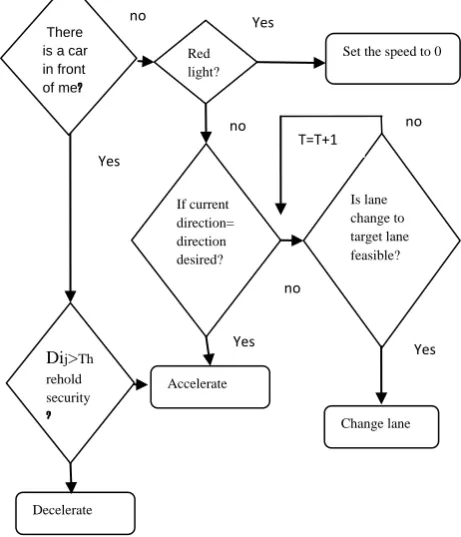
Bierly(1963) af(t+t)= [vL(t)-vf(t)] +[xL(t)-xf(t)] Bexeluis (1968) af(t+t)= [vL(t)-vf(t)] +[vt(t)-xf(t)] In microscopic models, traffic is described at the level of individual vehicles and their interaction among each other. Normally, this behavior is captured in some set of rules which determine when a vehicle accelerates, decelerates, changes lane; in addition, it regulates how and when vehicles choose and change their routes according to their destinations, and how they react to traffic and route information along the way.
Red light?
Set the speed to 0
Change lane Is lane change to target lane feasible? If current
direction= direction desired?
Decelerate Dij>Th rehold security ?
Accelerate Yes
no Yes
no
no
Yes Yes
no T=T+1
There is a car in front
of me?
T0i=T0i-1-(lnU)/ and V0i= Vem + σv*(-2Ln(U1))1/2*cos(2πU2)
t, P(N𝑡 + − Nt = 1) = . h + o(h) quand h → 0
[image:3.595.313.544.472.741.2] t, P(Nt + h − Nt > 1) = 𝑜() 𝑞𝑢𝑎𝑛𝑑 → 0
[image:3.595.59.278.476.714.2]In the first case, the vehicles are distributed randomly on the network according to the distribution model defined for each junction of the network. The vehicles react to the information concerning their next action. Models differ according to the various answers to the key questions: What is the nature of the action adequate ? To what stimulus it does react? and how to measure the characteristics of the other agents? The first and simplest model correspond to the case when the response is represented by the acceleration or deceleration of the vehicle.
4.
THE COMBINATION OF THE NEW
MODEL AND AIMSUN2
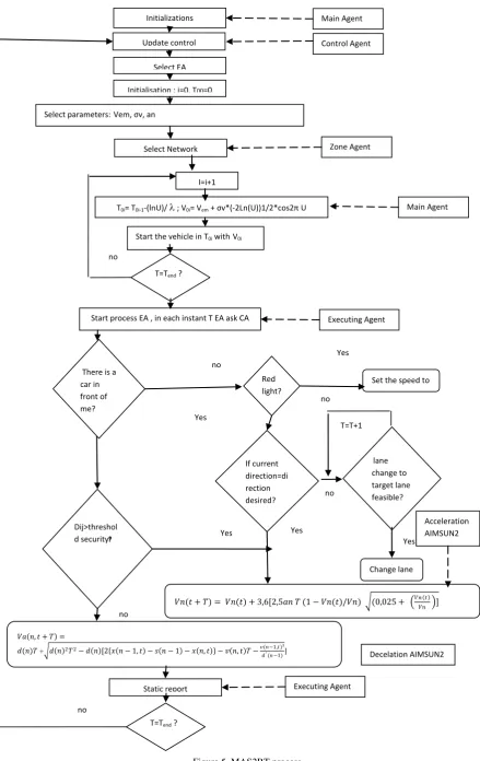
In this section, the proposed hybrid method incorporates the AIMSUN2 process , especially the equation of acceleration and deceleration, whose performance and results in practice proved valid and credible. AIMSUN2 (Ferrer & Barceló, 1994) was one of the first microscopic models ever developed; it aims to create a tool that could reproduce the dynamic aspects of traffic modeling and provides a very detailed road network.
According to Gipps [21 ] in the AIMSUN2 , the speed of the vehicle i-1 is controlled by three conditions. The first condition ensures that the vehicle does not exceed the average speed . The second condition ensures that the vehicle is accelerated to the desired speed with a rate of acceleration which increases the initial speed. The third condition ensures the decrease of the vehicle speed to zero as it approaches the desired speed. The combination of these conditions results in equation (1) If Xn(t) and Xn+1(t) are the positions of the leader and follower respectively at time t then:
Taking into consideration this equation, (Gipps, 1981), (Mahut, 2000)[26], develops an empirical model consisting of two components: acceleration and deceleration defined as a function of variables that can be measured. The first represents the intention of a vehicle to achieve certain desired speed; while, the second reproduces the limitations imposed by the preceding vehicle when trying to drive at the desired speed. This model states that the maximum speed a vehicle (n) can accelerate during a time period (t, t+T) is given by:
Where Vn(t) is the speed of vehicle at time t (km/h); an is the maximum desired acceleration rate of vehicle n (m/s); T is the driver’s reaction time (s); and Vn is the desired speed of vehicle n or the vehicle-specific free-flow speed (km/h).
The limitation imposed by the presence of the leader vehicle is:
Where: d (n) (< 0) is the maximum deceleration desired by vehicle n; x (n, t) is position of vehicle n at
time t; x (n-1, t) is position of preceding vehicle (n-1) at time t; s (n-1) is the effective length of vehicle
(n-1); d’ (n-1) is an estimation of vehicle (n-1) desired deceleration.
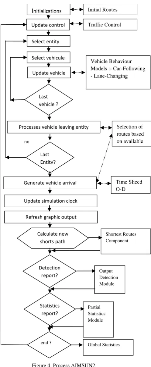
AIMSUN2 process is characterized by different types of traffic control including traffic light, the priority of the ways, and ramp metering. In this model see figure 4. In this sense, the new model (see figure 5) is based on the same process, except that inclusion of the distribution model and the interaction model. Both inserted models make the simulation more real and the results more eligible.
I
nitializationsUpdate control
Select entity
Select vehicule
Update vehicle
Generate vehicle arrival Last
vehicle ? ?
end ? no
Processes vehicle leaving entity
Last Entity?
Refresh graphic output Update simulation clock
Calculate new shortspath
Detection report?
Statistics report?
Initial Routes
Calculation
Traffic Control
M odels
Vehicle Behaviour Models :- Car-Following - Lane-Changing
Selection of routes based on available Information
Time Sliced O-D Matrices
Shortest Routes Component
Output Detection Module
Partial Statistics Module
Global Statistics
𝑉𝑛(𝑡 + 𝑇) = 𝑉𝑛(𝑡) + 3,6[2,5𝑎𝑛 𝑇 (1 − 𝑉𝑛(𝑡)/𝑉𝑛) (0,025 + 𝑉𝑛 𝑡 𝑉𝑛 ]
ẍ𝑛 + 1 𝑡 + 𝑇 =ẋ𝑛 𝑡 −ẋ𝑛 + 1 𝑡 𝑎𝑛𝑑
𝑖𝑓 ẋ𝑛(𝑡) < ẋ𝑛 + 1(𝑡) 𝑡𝑒𝑛 ẍ𝑛 + 1(𝑡 + 𝑇) < 0
𝑖𝑓 ẋ𝑛(𝑡) = ẋ𝑛 + 1(𝑡) 𝑡𝑒𝑛 ẍ𝑛 + 1(𝑡 + 𝑇) = 0
𝑖𝑓 ẋ𝑛(𝑡) > ẋ𝑛 + 1(𝑡) 𝑡𝑒𝑛 ẍ𝑛 + 1(𝑡 + 𝑇) > 0
𝑉𝑎 𝑛, 𝑡 + 𝑇 = 𝑑 𝑛 𝑇
+ 𝑑 𝑛 2𝑇2− 𝑑 𝑛 [2 𝑥 𝑛 − 1, 𝑡 − 𝑠 𝑛 − 1 − 𝑥 𝑛, 𝑡 − 𝑣 𝑛, 𝑡 𝑇]−𝑣(𝑛−1,𝑡)²𝑑′(𝑛−1)
(1)
)
(2)
)
(3)
[image:4.595.316.565.67.670.2])
Initializations
Update control
Select EA
Initialisation : i=0, T00=0
Select parameters:Vem, σv, an
rs Select Network
Start process EA , in each instant T EA ask CA
Red light?
Set the speed to 0
Change lane lane change to target lane feasible? If current
direction=di rection desired?
𝑉𝑛(𝑡 + 𝑇) = 𝑉𝑛(𝑡) + 3,6[2,5𝑎𝑛 𝑇 (1 − 𝑉𝑛(𝑡)/𝑉𝑛) (0,025 + 𝑉𝑛 𝑡 𝑉𝑛 ]
Dij>threshol d security?
Yes no
Yes
no
no
Yes
Yes no
There is a car in front of me?
T=Tend ?
Yes
T=T+1
Static report
T=Tend ? no
Main Agent
Control Agent
Zone Agent
Main Agent
Executing Agent
Executing Agent
Decelation AIMSUN2
Acceleration
AIMSUN2
no
𝑉𝑎 𝑛, 𝑡 + 𝑇 =
𝑑(𝑛)𝑇 + 𝑑 𝑛 2𝑇2− 𝑑 𝑛 [2 𝑥 𝑛 − 1, 𝑡 − 𝑠 𝑛 − 1 − 𝑥 𝑛, 𝑡 − 𝑣 𝑛, 𝑡 𝑇 −𝑣(𝑛−1,𝑡)² 𝑑′(𝑛−1)]
I=i+1
T0i= T0i-1-(lnU)/ ; V0i= Vem + σv*(-2Ln(U))1/2*cos2π U
[image:5.595.56.496.65.762.2]Start the vehicle in T0i withV0i
5. EXPERIMENT AND VALIDATION
In this section, in order to assess the performance of the proposed hybrid algorithm, a series of experiments is conducted to illustrate that the proposed distribution model and interaction model can improve the microscopic traffic simulation.
We present two sets of experimental results. Our first set of experiments examines the input speed of the vehicles in a section of the road; the second one evaluates the speed average in an interval of speed. Both sets of experiments are compared to the observed results during one hour of real interaction, see (table 2& table 3)
T Speed observed
(km/h)
Speed simulated(km /h)
T1 42 41,1119704
T2 51 51,3086948
T3 57 53,3598941
T4 43 39,3539766
T5 56 43,1623830
T6 55 40,9921566
T7 45 47,0093724
T8 39 47,5420921
T9 59 45,4179147
T10 50 48,9087991
T11 55 59,4983246
T12 52 45,4543754
T13 51 49,1936663
T14 46 41,370824
T15 43 48,3736373
T16 47 55,963108
T17 48 45,9071494
T18 52 45,7218993
T19 56 34,4250076
T20 58 40,1402877
In this experiment, 40KM\h is the average speed and 7KM\h is the standard deviation. In this experiment, the focus was only on the first twenty vehicles; the percentage of the vehicles speed is presented in table 3. The observation showed that the simulated speed is randomly distributed at the level of entry, which resembles the results observed in the reality.
Additionally, most of the values examined in table 1 are around the average speed; the speed of 90% of vehicles is between 4060KM\h and 60KM\h as shown in table 3.
Observed
values with speed
in[0-20[
v P(x=v)
0 0,0003
5 0,0001
10 0,003
15 0,006
values with speed in[20-40[
v P(x=v)
20 0,136581215
25 0,074285714
30 0,096418516
35 0,035914281
values with speed
in[40-60]
v P(x=v)
40 0,178571421
45 0,451153116
50 0,079428571 55 0 ,071428571
values with speed>60
v P(x=v)
65 0,12
70 0,09
75 0,02
80 0,0001
Our simulation
values with speed
in[0-20[
v P(x=v)
0 0
5 0,000833333
10 0,000785714
15 0,000416190
values with speed in[20-40[
v P(x=v)
20 0,006120071
25 0,024903007
30 0,046153146
35 0,190406111
values with speed
in[40-60]
v P(x=v)
40 0,269230769
45 0,176113007
50 0,006923017
55 0,20008795
values with speed>60
v P(x=v)
65 0,142857143
70 0
75 0
80 0
[image:6.595.57.349.234.672.2]Table 3 .percentage of vehicle’s speed
5.
CONCLUSION
This work discussed the randomly distributed simulation of the road traffic. It described the main aspects of the general computer simulation and the specific features of the computer simulation in the field of road traffic. The first section introduced the topic. The second section provided a general description of the proposed Multi-Agent architecture. The third section proceeded with the description of the main issues of the distribution model and the interaction model as well as the stochastic distribution model. To evaluate the efficiency of the distribution and interaction models, they were integrated In AIMSUN2 in section four. The obtained results in section five proved the effectiveness of the new model and its relevance to reality.
This research does by no means intend to provide a general or a comprehensive study of the issue; it is just an attempt to shed light on microscopic traffic simulation by adding new dimensions and layers of study. The final results of the this paper proved its efficiency and applicability in real life.
7. REFERENCES
[1] Qi Yang and Haris N.koutsopolos “a microscopic simulation for evaluation of dynamic traffic management systems “. transport res, c vol.4 n. 3, pp 113 129, 1996 [2] Shang Lei, Jiang Hanping and LU Huapu “RESEARCH
OF URBAN MICROSCOPIC TRAFFIC SIMULATION SYSTEM”. Proceedings of the Eastern Asia Society for Transportation Studies, Vol. 5, pp. 1610 - 1614, 2005 [3] B. van Arem,A.P. de Vos and M.J.W.A. “3Vanderschuren
The microscopic traffic simulation model”. TNO-report INRO-VVG 1997-02b
[4] José M Vidal “Fundamentals of Multiagent Systems with NetLogo Examples”. March 1, 2010
[5] Katia P. Sycara “Multiagent Systems”. AI magazine Volume 19, No.2 Intelligent Agents Summer 1998. [6] Howard M.Taylor Samuel Karlin “An IntroductionTo
Stochastic Modeling” 3rd edition
[7] Christel Geiss “Stochastic Modeling” October 21, 2009 [8] Brian Brewingto, RobertGray, Katsuhiro Moizumi,
DavidKotz George Cybenk and Daniela Rus“Mobile agents in distributed information retrieval” Chapter 15, pages 355-395, in "Intelligent Information Agents", edited by Matthias Klusch
[9] Johan Janson Olstam, Andreas Tapani “Comparison of Car-following models”. VTI meddelande 960A • 2004 E-58195 Linköping Sweden
[10]Robert M. Itami “Simulating spatial dynamics: cellular automata theory” .Landscape and Urban Planning 30 ( 1994) 27-47
[11]Madeleine Brettingham “Artificial intelligence” TES Magazine on 1 February, 2008
[12]Martin L. Griss, Ph.D “ Software Agents as Next Generation Software Components” Chapter 36 in Component-Based Software Engineering: Putting the
Pieces Together, Edited by George T.Heineman, Ph.D. & William Councill, M.S., J.D., May 2001, Addison-Wesley [13]Stan Franklin and Art Graesser Is “ It an Agent, or Just
a Program?: A Taxonomy for Autonomous Agents” Institute of Intelligent Systems, University of Memphis, Memphis, TN 38152, USA
[14]Nick Jennings and Michael Wooldridge “Software Agents” IEE Review, January 1996, pp 17-20
[15]Kinzer, John P., Application of the Theory of Probability to Problems of Highway Traffic, thesis submitted in partial satisfaction of requirements for degree of B.C.E., Polytechnic Institute of Brooklyn, June 1, 1933. Abstracted in: Proceedings, Institute of Traffic Engineers, vOl. 5, 1934, pp. ii8-124.
[16]Adams, William F., "Road Traffic Considered as a Random Series," journal Institution of Civil Engineers, VOL 4, Nov.,'1936, pp. 121-13
[17]Greenshields, Bruce D.; Shapiro, Donald; Ericksen, Elroy L., Traffic Per-formance at Urban Street Intersections, Technical Report No. i, Yale Bureau of Highway Traffic, 1947.
[18]Mansoureh Jeihani, Kyoungho Ahn, Antoine G. Hobeika, Hanif D. Sherali, Hesham A.Rakha "Comparison Of TRANSIMS' Light Duty Vehicle Emissions With On-Road Emission Measurements" Transportation Research ISSN 1046-1469
[19] J.Barceló, J.L Ferrer, R Martı́n"Simulation assisted design and assessment of vehicle guidance systems " International Transactions in Operational Research Volume 6, Issue 1, January 1999, Pages 123–143
[20]Yu, LYue, PTeng, H "COMPARATIVE STUDY OF EMME/2 AND QRS II FOR MODELING A SMALL COMMUNITY" Transportation Research Record Issue Number: 1858 ISSN: 0361-1981
[21]P. G. Gipps "A behavioural car-following model for computer simulation" Transportation Research vol. 15, no. 2, pp. 105-111, 1981 DOI: 10.1016/0191-2615(81)90037-0 [22] Adams w,f.(1936).’road traffic considered as a random
serie’ j.instn.civ.enrgs.,4,121-13
[23] Greenberg, B. S., R. C. Leachman, and R. W. Wolff, "Predicting Dispatching Delays on a
[24] Low Speed, Single Track Railroad," Transportation Science, Vol. 22, No. 1, pp. 31-38, 1988.
[25] Heidemann D., A queuing theory approach to speed-flow-density relationships, Proc. Of the 13
[26] Th International Symposium on Transportation and Traffic Theory, France, July 1996.
[27] N.H. Minsky. The imposition of protocols over open distributed systems. IEEE Transactions on Soft-ware Engineering, February 1991.
[28] Ferber. J. Les systèmes multi-agents. Vers une intelligence collective. InterEditions, Paris, 1995.