Routing with Congestion Control in Computer Network
using Neural Networks
Abdulkareem Y. Abdalla
Computer Science Dept. University of Basrah,
Basrah, Iraq
Turki Y. Abdalla
Computer Engineering Dept. University of Basrah,
Basrah, Iraq
Khloud A. Nasar
Computer Science Dept. University of Basrah,
Basrah, Iraq
ABSTRACT
The neural networks are widely used to solve the routing problem and to manage the congestion in the computer networks. In this paper, two methods are proposed to solve this problem. In the first method a feed forward neural network is included in a central node to determine the complete path between any pair of nodes (source, destination). In the second method a routing approach consists of two feed forward neural networks is suggested to solve the routing problem with congestion control. The proposed methods are applied for typical examples of computer networks. Results of the testing show good performance.
Keywords
: Routing, congestion control, computer network, neural network.1. INTRODUCTION
In a communication network information is transferred from one node to another as data packets. Packet routing is a process of sending a packet from its source node (s) to its destination node (d). On its way, the packet spends some time waiting in the queues ofintermediate nodes while they are busy processing the packets that came earlier. Thus the delivery time of the packet, defined as the time it takes for the packet to reach its destination, depends mainly on the total
time it has to spend in the queues of the intermediate nodes. Normally, there are multiple routes
that packet could take, which means that the choice of the route is crucial to the delivery time of the packet for any (source, destination) pair [1]. Routing algorithms are methods for finding the best way from a node s to another node d. This may be via a large number of other nodes or it may be in the next sub network. On a small, simple network the problem is almost trivial, statically allocating routes and defining them by hand, but when dealing with a huge internetwork such as the Internet this is not possible. Calculating the best route through such a complex system is computationally difficult and impossible to do by hand [2 , 3, 4].
If part of network becomes over_ filled with packets it can become impossible for packets to move. The queues into which they would be accepted are always full. This is called congestion. Routing algorithms strongly related to congestion [2, 5].
2. ROUTING USING NEURAL
NETWORKS
The routing problem defined by determining the optimal route for a packet from source node to destination node. The routing
decision must be made under the network current conditions such that traffic load, congestion and node or link failures.
Using the conventional algorithms and particular
mathematical programming methods to solve this problem is not recommended for practical purposes. Because, their calculations may take long time, which may leads to slowly response of the networks.
The parallel, distributed processing structure of the neural networks and their ability to learn are justified to use it as a structure for solving the routing problem. As a result, neural networks are considered to solve such kind of optimization problem. Optimal route is obtained by routing decision which is based on observed delay function. Also, for local decision routing, neural network at each node of computer network use just local information to decide to which neighbor node should be send the packet in order to reach its destination quickly [4, 6, 7].
3. CONGESTION CONTROL USING
NEURAL NETWORKS
One of the major problems for most communications networks lies in defining an efficient packet routing policy. Routing policy should be able to take into account the congestion. It sends the packet through route that may be long in terms of hops but results in shorter delivery time [1, 4]. The aim of the good routing algorithm is to minimize the effect of network congestion. But, the main problem of conventional routing algorithms that if costs are assigned in a dynamic way, based on statistical measures of the link congestion state, a strong feedback effect is introduced between the routing policies and the traffic patterns. This can lead to undesirable oscillations [5].
A. Rahmani [12] implement a new queuing mechanism in the intermediate routers, to control and avoid congestion. A. Dana and N. Salehi [13] propose a routing algorithm for choosing the channel that has more free-slots input buffer beyond adjacent routers.
4. PROPOSED METHODS
This paper presents our proposed approaches based on using neural networks to solve the routing problem and to manage the congestion in a context of computer networks.
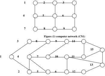
The computer networks which are considered in this paper modeled as graphs. Two examples, the first is a 9- node mesh computer network (CN1) shown in Figure (1). While the second is a random computer network (CN2) shown in Figure (2). The values of cost of the links (packet delay) and queue length of the nodes for these two computer networks are shown in Tables (1) and (2), respectively. The values of the queue lengths in these Tables are changing continuously, when the nodes send or receive the packets.
1
2
3
4 5 6
7 8 9
Figure (1) computer network (CN1)
3 8 9 14
15
1 4 7 10 11
13
2 5 6 12
Figure (2) computer network (CN2) Table (1) link costs and queue lengths of the computer network (CN1) Links Nodes link cost(packet delay) (in second) node queue length (in packet) 1__ 2 10 1 6
1__ 4 2 2 5
2__ 3 3 3 8
2__ 5 15 4 4
3__ 6 8 5 7
4__ 5 2 6 7
4__ 7 1.6 7 4
5__ 6 1.2 8 6
5__ 8 2.1 9 6
[image:2.595.82.433.205.461.2] [image:2.595.196.401.519.771.2]Table (2) link costs and queue lengths of the computer network (CN2)
Links Nodes
link
cost (packet
delay) (in second)
node queue length
(in packet)
1__ 2 6.312 1 5
1__ 3 6.312 2 5
2__ 4 1.544 3 7
2__ 5 6.312 4 7
3__ 8 6.312 5 4
4__ 5 3.352 6 8
4__ 7 6.312 7 8
4__ 8 3.352 8 5
5__ 6 12.624 9 6
6__ 10 3.352 10 5
6__ 12 6.312 11 4
7__ 9 3.152 12 6
7__ 10 3.152 13 3
8__ 9 6.312 14 4
9__ 14 12.624 15 6
10__ 11 3.152 10__ 13 3.152
11__ 14 3.152 11__ 15 3.152
12__ 13 6.312
13__ 15 6.312
14__ 15 6.312
4.1. Routing Decision
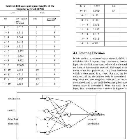
In this method, a recurrent neural network (NN1) is suggested which has M + 2 inputs, they are source, destination and M inputs for the link time costs, where M is the total number of the links in the computer network. The output is a sequence of nodes of the best path (n1 n2 ... nr) from destination to source which is determined in r_ steps. For that, the best neighbor node (n1) of the destination node is determined at the first step, then the best neighbor node (n2) to the node (n1) is determined, and so on, until the best neighbor node (nr) to the source node is determined. With ten units in one hidden layer. This neural network is shown in Figure (3).
destination
source
best neighbor
M of link node of
time costs
destination
Figure (3) the recurrent neural network (NN1)
In this method one neural network is used. It is included at a central node of the computer network to determine the best path to send packet from source node to destination node. When it receives information about the source, the destination and time costs of the links in the computer network, it makes routing decision which takes many iterative steps. First, it decides the best neighbor node of the
destination node. Then, this neighbor node becomes the new destination, and the neural network decides the best neighbor node of this new destination node, and so on, until it decides the best neighbor node of the source node. For example, in the computer network (CN1), for determining the best path to send packet from node 7 to node 3, the neural network (NN2) at the central node receives source 7, destination 3 and time costs of all links in the computer network (CN1). It decides that node 2 is the best neighbor node of destination 3,
node 1 is the best neighbor node of node 2 and node 4 is the best neighbor node of node 1.
4.2. Routing and Congestion
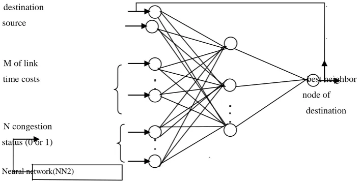
Control
For solving the routing problem with congestion control. Routing system is suggested which consists of two feed forward neural networks. The first, a feed forward neural network (NN2) has 3N inputs that represent average number of packets, variance of packets and polling flag of sending packets for N nodes, where N is the number of nodes in the computer network, and N outputs, represent numbers (as 0 or 1) to indicate congestion status of network nodes, with N units in one hidden layer. This neural network has connections between input layer and hidden layer
[image:3.595.64.501.57.539.2] [image:3.595.326.535.71.217.2]N of average
numbers of packets
N congestion
N of variances
status (0 or 1)
of packets
N of polling flags
of sending packets
Figure (4) the feed forward neural network (NN2)
each node is neighbor to itself. That instead of providing a fully connected environment. Figure (4)
The second part, is a recurrent neural network (NN3), has N + M + 2 inputs, they are source, destination, M of link time costs and N
the number of links in the computer network. The output is a sequence of nodes of the best path from destination to source which is determined in r_ steps. With ten units in its one hidden layer. Figure (5) view this neural network.
destination
source
M of link
time costs
best neighbor
node of
destination
N congestion
status (0 or 1)
Neural network(NN2)
Figure (5) the recurrent neural network (NN3)
The computer network has this routing system at a central node. The neural network (NN2) is worked
as congestion predictor, it receives the statistics (average number of packets, variance of packets and polling flag of sending packets) of all network nodes and determines the congestion status of them. The congestion status are represented as (0 or 1) numbers, where 0 for non congested nodes and 1 for congested nodes.
The neural network (NN3) is responsible to make routing decision for sending a packet from source node to destination node. It receives source, destination, the time costs of all network links and the output of congestion predictor (NN2) as congestion status of all network nodes. Then, it takes several iterative steps to determine the non congested nodes of the best path. At the beginning, the best neighbor node of the destination node is determined, after that, this best node before the destination node becomes the
determined. When all the neighbor nodes of a certain node in the path are congested, the neural network (NN3) selects the best one of them, that has the best link time cost for sending packet to it.
[image:4.595.63.460.79.260.2] [image:4.595.75.429.355.534.2]4.3. Simulation Result
In order to test the proposed methods, they are applied for two examples of computer networks (CN1, CN2) shown in Figures (1) and (2). The implementation of the simulation has been realized using C++ programming language.
The activation function used of these feed forward
neural networks is a sigmoid function as in equation:
)
1
(
1
1
)
(
xe
x
f
where λ is a size of step, λ ≥ 0. Where real numbers are used to represent their inputs and outputs.
Table (3) describe the number of inputs, outputs and hidden units of these neural networks. At this Table, N is the number of nodes and M is the number of links in the computer network, and r is the number of iteration steps of the recurrent neural network for determining the best path of packet
from source node to destination node. Where N = 9, M=2 for the computer network (CN1) and N = 15, M = 22 for the computer network (CN2).
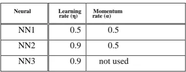
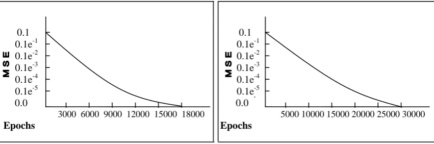
For all feed forward neural networks, the training sets and the test sets are prepared. The training set consists of the inputs of the neural network, for example source node, destination node, link costs and queue lengths, and the desired outputs, such as best neighbor node, best path from source to destination. In training stage, random values between – 0.5 and 0.5 are used as initial weights of connections of the neural networks. The neural networks are trained on 30 training sets with the back propagation algorithm for each computer networks (CN1, CN2). For any set, the training is continued until the mean squared error (MSE) becomes acceptable. The neural networks are trained on all possible routing decisions. In this stage, values of learning rate (η) and momentum rate (α) are selected by trial and error, which are given in Table (4). The obtained results are shown in Figures (6)_ (11). These Figures view mean squared error versus number of epochs, where this error is decreased when number of epochs is increased.
Then, testing the performance of these neural networks is performed on the trained sets, and on other test sets which are unseen before. Tables (5)_ (8) exposes some results of the testing of computer networks (CN1, CN2).
Through the testing of the proposed feed forward neural networks, results show their good performance, as observed in Tables (9) and (10) for computer networks (CN1, CN2), respectively. These Tables describe the success rates to test trained sets and test sets.
Table (3) the number of inputs, outputs and hidden units of the proposed feed forward neural networks
Neural
network
Number of
inputs Number of outputs
Number of hidden units
NN1
M + 2 1 (r steps) 10
NN2 3N N N
NN3
N + M + 2 1 (r steps) 10
Table (4) learning rates and momentum rates of the proposed feed forward neural networks
Neural
network
Learning
rate (η)
Momentum rate (α)
NN1 0.5 0.5
NN2 0.9 0.5
[image:5.595.316.540.224.329.2] [image:5.595.333.524.380.454.2]
0.1
0.1
0.1e-1 0.1e-1 0.1e-2 0.1e-2 0.1e-3 0.1e-3 0.1e-4 0.1e-4 0.1e-5 0.1e-5
0.0 0.0
3000 6000 9000 12000 15000 18000 5000 10000 15000 20000 25000 30000
Epochs
Epochs
Figure (6) error versus number of epochs of Figure (7) error versus number of epochs of the feed forward neural network (NN1) for the the feed forward neural network (NN1) for the computer network (CN1) computer network (CN2)
0.1
0.1
0.1e-1 0.1e-1 0.1e-2 0.1e-2 0.1e-3 0.1e-3 0.1e-4 0.1e-4 0.1e-5 0.1e-5
0.0 0.0
200 400 600 800 1000 1200 300 600 900 1200 1500 1800
Epochs
Epochs
Figure (8) error versus number of epochs of Figure (9) error versus number of epochs of the feed forward neural network (NN2) for the the feed forward neural network (NN2) for the
computer network (CN1) computer network (CN2)
0.1
0.1
0.1e-1 0.1e-1 0.1e-2 0.1e-2 0.1e-3 0.1e-3 0.1e-4 0.1e-4 0.1e-5 0.1e-5
0.0 0.0
4000 8000 12000 16000 20000 24000 5500 11000 16500 22000 27500 33000
Epochs
Epochs
[image:6.595.56.482.79.220.2] [image:6.595.56.485.324.466.2] [image:6.595.60.482.564.705.2]
Table (5) The test results of the feed forward neural network (NN1) for the computer network (CN1)
Source Destination
Best path Outputs of the
recurrent (NN1)
8
2 ( 8 5 6 3 2 ) ( 3 6 5 ) 2 9 ( 2 5 8 9 ) ( 8 5 )
3 7 ( 3 2 1 4 7 ) ( 4 1 2 )
9 2 ( 9 6 3 2 ) ( 3 6 )
1 9 ( 1 4 5 8 9 ) ( 8 5 4 )
3 5 ( 3 6 5 ) ( 4 1 2 )
Table (6) Test results of the feed forward neural network (NN1) for the computer network (CN2)
Source
Destination Best path
Outputs of the recurrent (NN1)
13 2 ( 13 10 7 4 2 ) ( 4 7 10 )
11 4 ( 11 10 7 9 8 4 ) ( 8 9 7 10 )
1 8 ( 1 2 4 8 ) ( 4 2 )
2 13 ( 2 4 7 10 13 ) ( 10 7 4 )
4 9 ( 4 7 9 ) ( 7 )
8 15 ( 8 9 14 15 ) ( 14 11 10 7 9 )
Table (7) some of the test results of the feed forward neural network (NN3) for the computer network (CN1)
Source Destination
Outputs of the
Congestion predictor
(NN2)
Best Path
Outputs of the recurrent neural
Network(NN3)
network (NN2)
7 6 ( 1 0 0 0 0 0 0 0 1 ) ( 7 4 5 6 ) ( 5 4 )
2 9 ( 0 0 0 0 1 0 0 1 0 ) ( 2 3 6 9 ) ( 6 3 )
3 7 ( 0 0 0 0 1 1 1 0 0 ) ( 3 2 1 4 7 ) ( 4 1 2 )
6 7 ( 0 0 0 0 0 0 0 0 0 ) ( 6 5 4 7 ) ( 4 5 )
8 3 ( 1 0 0 0 0 0 0 0 1 ) ( 8 5 2 3 ) ( 2 5 )
1 5 ( 0 0 0 1 0 0 0 0 0 ) ( 1 2 5 ) ( 4 )
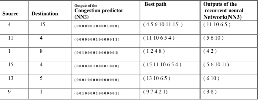
Table (8) some of the test results of the feed forward neural network (NN3) for the computer network (CN2)
Source Destination
Outputs of the
Congestion predictor (NN2)
( NN2)
Best path Outputs of the recurrent neural
Network(NN3)
network (NN3)
network (NN2)
4 15 ( 0 0 0 0 0 0 1 0 0 0 0 1 0 0 0 ) ( 4 5 6 10 11 15 ) ( 11 10 6 5 )
11 4 ( 0 0 0 0 0 0 0 1 0 0 0 0 0 1 1 ) ( 11 10 6 5 4 ) ( 5 6 10 )
1 8 ( 0 0 1 0 0 0 0 1 0 0 0 0 0 0 1) ( 1 2 4 8 ) ( 4 2 )
15 4 ( 0 0 0 0 0 0 1 0 0 0 0 1 0 0 0 ) ( 15 11 10 6 5 4 ) ( 5 6 10 11)
13 5 ( 0 0 0 1 0 0 0 0 0 0 0 0 0 0 0 ) ( 13 10 6 5 ) ( 6 10 )
9 1 ( 0 0 1 0 0 0 0 1 0 0 0 0 0 0 1 ) ( 9 7 4 2 1) ( 3 8 )
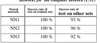
[image:7.595.41.545.76.277.2] [image:7.595.48.477.316.494.2] [image:7.595.50.479.528.695.2]Table (9) success rates of testing the proposed neural networks for the computer network (CN1)
Neural
network
Success rate of
test on trained sets Success rate of test on other sets
NN1 100 % 93 %
NN2 100 % 96 %
NN3 100 % 92 %
Table (10) success rates of testing the proposed neural networks for the computer network(CN2)
Neural
network
Success rate of
test on trained sets Success rate of test on other sets
NN1 100 % 92 %
NN2 100 % 94 % NN3 100 % 90 %
5.
CONCLUSION
This paper introduces the description of two proposed methods using neural networks for solving the routing problem and control the congestion in computer networks. The recurrent neural networks (NN1, NN3) use universal information of the computer network to determine the complete path from the source node to the destination node. The feed forward neural network (NN2) which works as congestion predictor has number of inputs, outputs and hidden units that dependon the number of nodes of the computer network. Simulation results obtained, when the proposed methods were applied for two different examples of computer network structures show good performance, in making routing decision and manage the congestion problem.
6. REFRENCES
[1] S. Kumar and R. Miikkulainen, “ Confidence_ Based Q_ Routing: An On_ Line Adaptive Network Routing Algorithm ”, Proceedings of the Artificial Neural Networks in Engineering Conference, Texas University, Austin, 1998.
[2] D. Davies, D. Barber, W. Price and C. Solomonides, “ Computer Networks and Their Protocols”, J. Wiley and Sons Ltd, New York, 1979.
[3] J. Malrand, “ Communication Networks: A First Course ”, R. D. Irwin and Akson Associates, Inc, 1991.
[4] W. Newton, “ A Neural Network Algorithm for Internetwork Routing ”, Report in Software Engineering, for Degree of Bachelor, 2002.
[5] G. Caro and M. Dorigo, “ AntNet: A Mobile Agents Approach to Adaptive Routing ”, Technical Report, Iridia University, No. 12, 1997.
[6] C. Tseng and M. Garzon, “ Hybrid Distributed Adaptive Neural Router ”, Texas University, USA, 1996, E_ mail: [email protected].
[7] J. Menke, “ Distributed Neural Network Routing ”, Proceeding of the ANNIE, 1999.
[8] J. Bivens, B. Szymanski and M. Embrechts, “ Network Congestion Arbitration and Source Problem Prediction Using Neural Networks ”, Smart Engineering System Design, Vol. 4, 2002.
[9] I. Glauche, W. Krause, R. Sollacher and M. Greiner, “ Distributive Routing and Congestion Control in Wireless Multihop Ad_ hoc Communication Networks ”, Elsevier Science, arXiv: cond_ mat No. 0404434 V1, 19 April, 2004.
[10] S. Dimitrov, M. Epelman and D. Sharama, “ New Models of Network Routing under Active Congestion Control ”, Michigan University, Industrial and Operations Engineering Department, 2009.
[11] M. Proebster, M. Schart and S. Hauger, “ Performance Comparison of Router Assisted Congestion Control Protocols: XCP vs. RCP ”, Stuttgart University, Germany, 2009.
[12] A. Bidgoli, A. Bahri and A. Rahmani,“ Differentiated
Services Fuzzy Assured Forward Queuing for
Congestion Control in Intermediate Routers ”, Islamic Azad University, Iran, 2011.
[image:8.595.48.255.93.183.2]