Non Linear Feedback Neural Network for Solution of Quadratic Programming Problems

Non-linear Feedback Neural Network for Solution of

Quadratic Programming Problems

Mohd. Samar Ansari

Department of Electronics Engineering Aligarh Muslim University

Aligarh, India

Syed Atiqur Rahman

Department of Electronics Engineering Aligarh Muslim University

Aligarh, India

ABSTRACT

This paper presents a recurrent neural circuit for solving quadratic programming problems. The objective is tominimize a quadratic cost function subject to linearconstraints. The proposed circuit employs non-linearfeedback, in the form of unipolar comparators, to introducetranscendental terms in the energy function ensuring fastconvergence to the solution. The proof of validity of the energy function is also provided. The hardware complexity of the proposed circuit comparesfavorably with other proposed circuits for the same task. PSPICE simulation results arepresented for a chosen optimization problem and are foundto agree with the algebraic solution.

General Terms

Neural Networks, Quadratic Programming Problem.

Keywords

Dynamical Systems, Non-Linear Synapse, Feedback Networks.

1.

INTRODUCTION

Quadratic programming problem (QPP) is the problem of optimizing (minimizing or maximizing) a quadratic function of several variables subject to linear constraints on these variables. Such problems arise naturally in a variety of applications, such as structural analysis [1], optimal control [2], plastic analysis [3], antenna array pattern synthesis [4], geometric optimization [5], propulsion physics [6], multi-commodity networks [7], etc. Moreover, in the discipline of constrained optimization, problems with nonlinear objective functions are usually approximated by a second-order system and solved by a standard quadratic programming technique. Traditional methods for solving quadratic programming problems typically involve an iterative process, but long computational time limits their usage. An alternative approach to solution of this problem is to exploit the artificial neural networks (ANN's) which can be considered as an analog computer relying on a highly simplified model of neurons [8]. ANN's have been applied to several classes of constrained optimization problems and have shown promise for solving such problems more effectively. For example, the Hopfield neural network has proven to be a powerful tool for solving some of the optimization problems. Tank and Hopfield first proposed a neural network for solving mathematical programming problems, where a linear programming problem (LPP) was mapped into a closed-loop network [9]. Later, the dynamical approach was extended for solving quadratic programming problems. Over the past two decades several neural-network architectures for solving quadratic programming problems have been proposed by Kennedy & Chua [10], Maa&Shanblatt[11], Chen & Fang [12], Wu et

al.[13] and Xia [14]. More recently, Malek&Alipour proposed a recurrent neural network that is able to solve quadratic programming problems [15] without needing to set network parameters thereby reducing the number of analog multipliers required.

In this paper, a hardware solution to the problem of solving a quadratic programming problem is presented. The proposed architecture uses non-linear feedback which leads to a new energy function that involves transcendental terms. This transcendental energy function is fundamentally different from the standard quadratic form associated with Hopfield network and its variants. To solve a QPP in n variables with m constraints, the circuit requires n opamps,m unipolar comparators and (n2+mn) resistances thereby causing the hardware complexity of the proposed network to compare favorably with the existing hardware implementations. It may be mentioned that a similar approach of using non-linear synaptic interconnections between neurons has also been employed to solve systems of simultaneous linear equations [16] and linear programming problems [17].

The remainder of this paper is arranged as follows. A brief review of relevant technical literature on the solution of QPP using neural network based methods is presented in Section-2. Section-3 outlines the mathematical formulation of the basic problem and details of the proposed network. Section-4 contains explanation of the energy function and the proof of its validity. Section-5 contains the circuit implementation of the proposed network for a set of sample problem in two variables. PSPICE simulation results of the proposed circuit are also presented. Issues that are expected to arise in actual monolithic implementations are discussed in Section-6. Concluding remarks are presented in Section-7.

2.

EXISTING NEURAL NETWORKS

FOR QPP

of the network is also presented which requires (n+m) neurons for solving a QPP in n variables with m constraints. Each neuron is made up of a summer, an integrator, and an inverter consuming 3 opamps, 1 capacitor and (n+5) resistors [18]. Wang's network is not suitable for real time applications as it takes around 50 ms to arrive at the solution [18]. A rigorous analysis of the prominent neural networks for QPP, available till that time (1992), is presented in [11]. Forti&Tesi presented new conditions capable of ensuring existence, uniqueness, and global asymptotic stability of the equilibrium point for Kennedy and Chua's network [19]. Wu et al. proposed two neural network models for solving LPP and QPP, the convergence of which was not dependent on the network parameters [13].

Around the same time, Xia also put forward a neural network capable of solving both LPP and QPP in which no parameter tuning was necessary. Moreover, the actual hardware implementation was somewhat simplified, as compared to its contemporaries, because of the fact that no analog multipliers were required for the variables [14]. To solve a QPP in n variables with m constraints, Xia's network consisted of (2m2+4mn) amplifiers, (2m2+4mn+3m+3) summers, (n+m) integrators, and n limiters. Tao, Cao and Sun further simplified the network of Xia [14], and reduced the system complexity [20]. More recently, Liu and Wang presented a one layer feedback neural network with a discontinuous hard-limiting activation function for solving QPP in which the number of neurons is the same as the number of decision variables [21]. Each neuron in [21] is composed of two adders, (3n+1) resistors, one limiter and an integrator. Although significant reduction in circuit complexity is achieved, the time that the circuit takes to arrive at the correct solution is of the order of seconds thereby making the circuit unsuitable for applications requiring fast solution times. A comprehensive bibliography of the technical literature related to QPP can be found in [22].

3.

PROPOSED CIRCUIT

Let the second-orderfunction to be minimized be

𝐹 = 𝑉1

𝑉2

⋮ 𝑉𝑛

𝑇 _c

11 c12 … c1n

c21 c22 … c2n

⋮ ⋮ … ⋮

cn1 cn2 … cnn

𝑉1

𝑉2

⋮ 𝑉𝑛

(1)

subject tothe following linear constraints

a11 a12 … a1n

a21 a22 … a2n

⋮ ⋮ … ⋮

am1 am2 … amn

𝑉1

𝑉2

⋮ 𝑉𝑛

≤ b1

b2

⋮ bm

(2)

whereV1, V2,…, Vn are the variables, and aij, cij and bi (i = 1, 2,

…, m; j = 1, 2, …, n) are constants. The proposed neuralnetwork based circuit to minimize the quadratic function given in (1) in accordance with the constraints of (2) is presented in Fig. 1. As can be seen from Fig. 1, individual equations from the set of equations to be solved are passed through non-linear synapses which are realized using unipolar comparators comprising of operational amplifiers and diodes. Rp1 and Cp1are the input resistance and capacitance of the

[image:2.595.316.543.72.224.2]

opamp that is used to emulate the functionality of a neuron. These parasitic components are included to model the dynamic nature of the opamp. The outputs of the comparators are fed to neurons having weighted inputs. The neurons are realized by using opamps and the weights are implemented using resistances. The currents arriving to the neuron from various synapses get added up at the input of the neuron.

Fig 1: First neuron of the proposed feedback neural network circuit to solve a quadratic programming

problem in n variables with m linear constraints.

Graphical representation of the transfer characteristics for a bipolar comparator is shown in Fig 2(a) from where it can be seen that the comparator output saturates at ±Vm when the two

[image:2.595.317.541.405.775.2]

inputs differ by more than few millivolts in magnitude. Unipolar transfer characteristics can be obtained using an opamp (the transfer characteristics of which can be modeled by (3) by employing a diode as depicted in Fig. 3, the diode essentially `trimming' one half of the transfer characteristic curve, which are shown in Fig. 2(b) and can be mathematically modeled by (4). As is explained in the next section, such unipolar comparator characteristics are utilized to obtain an energy function which acts to bring the neuronal states to the feasible region.

Fig 2: Transfer characteristics of (a) bipolar; and (b)unipolar; comparators

Fig 3: Obtaining unipolar comparator characteristics using an opamp and a diode

𝑥 = 𝑉𝑚𝑡𝑎𝑛ℎ 𝛽 𝑉𝑖− 𝑉𝑗 (3)

𝑥 =1₂𝑉𝑚 𝑡𝑎𝑛ℎ 𝛽 𝑉𝑖− 𝑉𝑗 + 1 (4) Using (4), the output of the i-th unipolar comparator in Fig. 1 can be given by (5) where βis the open-loop gain of the comparator (practically very high), ±Vm are the output voltage

levels of the comparator and V1, V2,…,Vn are the neuron

outputs.

[image:2.595.54.246.477.597.2]

Applying node equations for node ‘A’ in Fig. 1, the equation of motion of the i-th neuron can be given as

𝐶𝑖𝑑𝑢_𝑑𝑡𝑖= _𝑅𝑥1 𝑐1𝑖+

𝑥2

𝑅𝑐2𝑖+ ⋯ +

𝑥𝑛

𝑅𝑐𝑛𝑖

+ 𝑉1 𝑅1𝑖+

𝑉2

𝑅2𝑖+ ⋯ +

𝑉𝑛

𝑅𝑛𝑖 −

𝑢𝑖

𝑅𝑖 (6)

whereRi is the parallel equivalent of all resistances connected

at node ‘A’ in Fig. 1 and is given by

1

𝑅𝑖=

1 𝑅𝑗𝑖 𝑛

𝑗 =1

+ 1

𝑅𝑐𝑗𝑖 𝑛

𝑗 =1

+ 1

𝑅𝑝𝑖 (7)

whereui is the internal state of the i-th neuron, Rc1i, Rc2i, Rcni,

… are the weight resistance connecting the outputs of the unipolar comparators to the input of the i-th neuron and R1i,

R2i, Rni, … are the feedback resistances from the outputs of the

neurons to the input of the i-th neuron. As is shown later in this section, the values of these resistances are governed by the entries in the coefficient matrix of (2). Rpi and Cpi are the

input resistance and capacitance of the opamp corresponding to the i-th neuron.

Further, as has been explained in Section-3, the non-linear feedback neural circuit of Fig. 1 is associated with the following Lyapunov function (also referred to as the ‘energy function’)

𝐸 = 𝐶𝑖𝑗𝑉𝑖𝑉𝑗 𝑛

𝑗 =1 𝑛

𝑖=1

+𝑉𝑚

2 𝑎𝑖𝑗𝑉𝑗 𝑛

𝑗 =1 𝑚

𝑖=1

+ 𝑉𝑚

2𝛽 ln coshβ (𝑎𝑖𝑗𝑉𝑗 𝑛

𝑗 =1

− 𝑏𝑖) 𝑚

𝑖=1

(8)

This expression of the Energy Function can be written in a slightly different (but more illuminating) form as

𝐸 = 𝐶𝑗𝑖𝑉𝑖𝑉𝑗 𝑛

𝑗 =1 𝑛

𝑖=1

+ 𝑃1+ 𝑃2+ ⋯ + 𝑃𝑚 (9)

where the first term is the same as the second-order function to be minimized, as given in (1), and P1, P2, … , Pm are the

penalty terms. The i-th penalty term can be given as

𝑃𝑚 =

𝑉𝑚

2 𝑎𝑖𝑗𝑉𝑗

𝑛

𝑗 =1

+𝑉𝑚

2𝛽ln coshβ 𝑎𝑖𝑗𝑉𝑗− 𝑏𝑖

𝑛

𝑗 =1

(10)

Obtaining a partial differentiation of the combined penalty term, P (=P1+P2+…+Pm) with respect to Vi we have

𝜕𝑃 𝜕𝑉𝑖=

𝑉𝑚

2 𝑎𝑗𝑖

𝑚

𝑗 =1

+𝑉𝑚 𝛽 𝑎𝑗𝑖

𝑚

𝑗 =1

tanh β 𝑎𝑖𝑗𝑉𝑗 − 𝑏𝑖 𝑛

𝑗 =1

(11)

which may be simplified to

𝜕𝑃

𝜕𝑉𝑖 = 𝑎𝑗𝑖𝑥𝑗 𝑚

𝑗 =1

(12)

Using the above relations to find the derivative of the energy function E with respect to Vi we have

𝜕𝐸 𝜕𝑉𝑖 =

𝜕

𝜕𝑉𝑖 𝐶𝑖𝑗𝑉𝑖𝑉𝑗 𝑛

𝑗 =1 𝑛

𝑖=1

+𝜕𝑃

𝜕𝑉𝑖 (13)

which in turn yields

𝜕𝑃

𝜕𝑉𝑖= 𝑐𝑖𝑗 𝑛

𝑗 =1

+ 𝑎𝑗𝑖𝑥𝑗 𝑚

𝑗 =1

(14)

Also, if E is the Energy Function, it must satisfy the following condition [23]:

𝜕𝐸 𝜕𝑉𝑖= 𝐾𝐶𝑖

𝑑𝑢𝑖

𝑑𝑡 (15)

whereK is a constant of proportionality and has the dimensions of resistance. Equation (15) applied to the i-th neuron results in

𝑅𝑐𝑖𝑗 =

𝐾

𝑎𝑖𝑗 (16)

A similar comparison of the remaining partial fractions for the remaining variables yields the following:

𝑅𝑐11 𝑅𝑐12

𝑅𝑐21 𝑅𝑐22

… 𝑅𝑐1𝑛

… 𝑅𝑐2𝑛

⋮ ⋮

𝑅𝑐𝑚 1 𝑅𝑐𝑚 2

… ⋮

… 𝑅𝑐𝑚𝑛

= 𝐾

1 𝑎11 1 𝑎12

1 𝑎21 1 𝑎22

… 1 𝑎1𝑛

… 1 𝑎2𝑛

⋮ ⋮

1 𝑎𝑚1 1 𝑎𝑚2

… ⋮

… 1 𝑎𝑚𝑛

(17)

and

𝑅11 𝑅12

𝑅21 𝑅22

… 𝑅1𝑛

… 𝑅2𝑛

⋮ ⋮

𝑅𝑚1 𝑅𝑚2

… ⋮

… 𝑅𝑚𝑛

= 𝐾

1 𝑐11 1 𝑐12

1 𝑐21 1 𝑐22

… 1 𝑐1𝑛

… 1 𝑐2𝑛

⋮ ⋮

1 𝑐𝑚1 1 𝑐𝑚2

… ⋮

… 1 𝑐𝑚𝑛

(18)

4.

ENERGY FUNCTION

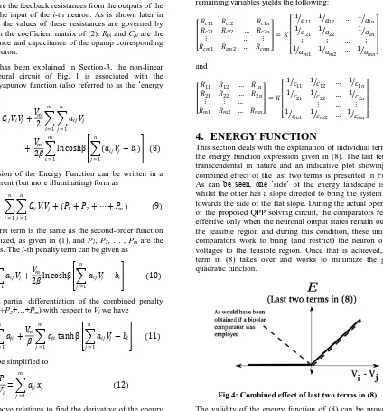
[image:3.595.99.523.243.698.2]

This section deals with the explanation of individual terms in the energy function expression given in (8). The last term is transcendental in nature and an indicative plot showing the combined effect of the last two terms is presented in Fig. 4. As can be seen, one ‘side’ of the energy landscape is flat whilst the other has a slope directed to bring the system state towards the side of the flat slope. During the actual operation of the proposed QPP solving circuit, the comparators remain effective only when the neuronal output states remain outside the feasible region and during this condition, these unipolar comparators work to bring (and restrict) the neuron output voltages to the feasible region. Once that is achieved, first term in (8) takes over and works to minimize the given quadratic function.

Fig 4: Combined effect of last two terms in (8)

The validity of the energy function of (8) can be proved as follows. The time derivative of the energy function is given by 𝑑𝐸 𝑑𝑡 = 𝜕𝐸 𝜕𝑉𝑖 𝑑𝑉𝑖 𝑑𝑡 𝑁 𝑖=1

= 𝜕𝐸 𝜕𝑉𝑖 𝑑𝑉𝑖 𝑑𝑢𝑖 𝑁 𝑖=1 𝑑𝑢𝑖

Using (15) in (19) we get

𝑑𝐸

𝑑𝑡 = 𝐾𝐶𝑖

𝑁

𝑖=1

𝑑𝑢𝑖

𝑑𝑡

2_𝑑𝑉 𝑖

𝑑𝑢𝑖 20

The transfer characteristics of the output opamp used to implement the neurons in Fig. 1 implements the activation function of the neuron and can be written as

[image:4.595.317.543.110.193.2]

𝑉𝑖= 𝑓 𝑢𝑖 21

Fig 5: Transfer characteristics of the opamp used to realize the neurons

whereVi denotes the output of the opamp and ui corresponds

to the internal state at the inverting terminal. The function f is typically a saturating, monotonically decreasing one, as shown in Fig. 5, and therefore [16],

𝑑𝑉𝑖

𝑑𝑢𝑖 ≤ 0 22

thereby resulting in

𝑑𝐸

𝑑𝑡 ≤ 0 23

with the equality being valid for

𝑑𝑢𝑖

𝑑𝑡 = 0 24

Equation (23) shows that the energy function can never increase with time which is one of the conditions for a valid energy function. The second criterion viz. the energy function must have a lower bound is also satisfied for the circuit of Fig. 1 wherein it may be seen that V1, V2, …, Vn are all bounded (as

they are the outputs of opamps, as given in (21) amounting to E, as given in (8), having a finite lower bound.

5.

SIMULATION RESULTS

This sectiondeals with the application of the proposed network to task of minimizing the objective function

3𝑉12+ 4𝑉1𝑉2+ 5𝑉22 25

subject to

𝑉1− 𝑉2≤ −1(26)

𝑉1+ 𝑉2 ≤ 1

The values of resistances acting as the weights on the neurons are obtained from (17,18). For the purpose of simulation, the value of K was chosen to be 1 KΩ. Using K = 1 KΩ in (17,18) gives

Rc11 = Rc12 = Rc21 = Rc22 = K = 1 K, R11 = 1.66 K, R21 = 1 K,

R12 = 1.66 K, R22 = 1 K

For the purpose of PSPICE simulations, the unipolar voltage comparator was realized using a diode clamp with an opamp based comparator. The transfer characteristics obtained during the PSPICE simulations for opamp based bipolar and unipolar comparators are presented in Fig.6. For the purpose of this

simulation, the LMC7101A CMOS opamp model from the Orcad library in PSPICE was utilised. The value of βfor this opamp was measured to be 1.1×104 using PSPICE simulation.

Fig 6: Transfer characteristics for opamp based unipolar and bipolar comparators

Routine mathematical analysis of (25) yields: V1= – 0.584,

V2= 0.416. The resultant plots of the neuron output voltages

[image:4.595.92.252.158.285.2]

as obtained after PSPICE simulation are presented in Fig.7 from where it can be seen that V(1) = –0.58 V and V(2) = 0.41 V which are very near to the algebraic solution thereby confirming the validity of the approach. The initial node voltages were kept as V(1) = –1 mV and V(2) = –10 mV.

Fig 7: Simulation results for the proposed circuit applied to minimize (25) subject to (26)

6.

ISSUES IN VLSI IMPLEMENTATION

This section deals with the monolithic implementation issues of the proposed circuit. The PSPICE simulations assumed that all operational amplifiers (and diodes) are identical, and therefore, it is required to determine how deviations from this assumption affect the performance of the network. Effects of variations in component values from one neuron to another were also investigated using Monte-Carlo analysis in PSPICE. A 10% tolerance with Gaussian deviation profile was put on the resistances used in the circuit to solve (25). The analysis was carried out for 100 runs and the Mean Deviation was found out to be -144.73×10-6 and Mean Sigma (Standard Deviation) was 0.0119. Offset analysis was also carried out by incorporating random offset voltages (in the range of 1 mV to 10 mV) to the opamps. The Mean Deviation in this case was measured to be -143.51×10-6and the Mean Sigma (Standard Deviation) was 0.012. As can be seen, the effects of mismatches and offsets on the overall precision of the final results are in an acceptable range.

[image:4.595.344.515.305.451.2]

Alternative realizations based on the differential equations (6) governing the system of neurons are being investigated. Other approaches to obtain the tanh(.) non-linearity include the use of a MOSFET operated in the sub-threshold region [24] and the use of Current Differencing Transconductance Amplifier (CDTA) to provide the same nonlinearity in the current-mode regime [25].

7.

CONCLUSION

In this paper, a CMOS compatible approach to solve a quadratic programming problem in n variables subject to mlinear constraints, which uses nneurons and msynapses is presented. Each neuron requires one opamp and each synapse is implemented using a unipolar voltage-mode comparator. This results in significant reduction in hardware over the existing schemes. The proposed network was tested on a sample problem of minimizing a quadratic function in 2 variables and the simulation results confirm the validity of the approach.

8.

REFERENCES

[1] Atkociunas, J. 1996. Quadratic programming for degenerate shakedown problems of bar structures. Mechanics Research Communications, 23(2), 195–206. [2] Bartlett, R.A., Wachter, A., and Biegler, L.T. 2000.

Active set vs. interior point strategies for model predictive control. In Proceedings of the American Control Conference, Chicago, USA, June 2000, 4229– 4233.

[3] Maier, G. and Munro, J. 1982. Mathematical programming applications to engineering plastic analysis. Applied Mechanics Reviews, 35, 1631–1643. [4] Nordebo, S., Zang, Z., and Claesson, I. 2001. A

semi-infinite quadratic programming algorithm with applications to array pattern synthesis. IEEE Transactions on Circuits and Systems II: Analog and Digital Signal Processing, 48(3), 225–232.

[5] Schonherr, S. 2002. Quadratic programming in geometric optimization: theory, implementation, and applications. Technical report, Swiss Federal Institute of Technology, Zurich.

[6] Borguet, S. and O. Lonard, O. 2009. A quadratic programming framework for constrained and robust jet engine health monitoring. Progress in Propulsion Physics, 1, 669–692.

[7] Dembo, R.S. and Tulowitzki, U. 1988. Computing equilibria on large multicommodity networks: An application of truncated quadratic programming algorithms. Networks, 18(4), 273–284.

[8] Krogh, A. 2008. What are artificial neural networks? Nature Biotechnology, 26(2), 195–197.

[9] Tank, D.W. and Hopfield, J. 1986. Simple ‘neural’ optimization networks: An A/D converter, signal decision circuit, and a linear programming circuit. IEEE Transactions on Circuits and Systems, 33(5), 533–541. [10]Kennedy, M.P. and Chua, L.O. 1988. Neural networks

for nonlinear programming. IEEE Transactions on Circuits and Systems, 35(5), 554–562.

[11] Maa, C.-Y. andShanblatt, M.A. 1992. Linear and quadratic programming neural network analysis. IEEE Transactions on Neural Networks, 3(4), 580–594. [12] Chen, Y.-H. and Fang, S.-C. 1998. Solving convex

programming problems with equality constraints by neural networks. Computers & Mathematics with Applications, 36(7), 41–68.

[13] Wu, X.-Y., Xia, Y.-S., Li, J., and Chen, W.-K. 1996. A high-performance neural network for solving linear and quadratic programming problems. IEEE Transactions on Neural Networks, 7(3), 643–651.

[14] Xia Y. 1996. A new neural network for solving linear and quadratic programming problems. IEEE Transactions on Neural Networks, 7(6), 1544–1548. [15] Malek, A. and Alipour, M. 2007. Numerical solution for

linear and quadratic programming problems using a recurrent neural network. Applied Mathematics and Computation, 192(1), 27–39.

[16] Rahman, S.A. and Ansari, M.S. 2011. A neural circuitwith transcendental energy function for solving system of linear equations. Analog Integrated Circuits and Signal Processing, 66, 433–440.

[17] Ansari, M.S. and Rahman, S.A. 2010. A DVCC-based non-linear analog circuit for solving linear programming problems. In Proceedings of International Conference on Power, Control and Embedded Systems (ICPCES), Dec 2010, 1–4.

[18] Wang, J. 1992. Recurrent neural network for solving quadratic programming problems with equality constraints. Electronics Letters, 28(14), 1345–1347. [19] Forti, M. and Tesi, A. New conditions for global

stability of neural networks with application to linear and quadratic programming problems. IEEE Transactions on Circuits and Systems I: Fundamental Theory and Applications, 42(7), 354–366.

[20] Tao, Q., Cao, J., and Sun, D. 2001. A simple and high performance neural network for quadratic programming problems. Applied Mathematics and Computation, 124(2), 251–260.

[21] Liu, Q. and Wang, J. 2008. A one-layer recurrent neural network with a discontinuous hard-limiting activation function for quadratic programming. IEEE Transactions on Neural Networks, 19(4), 558–570.

[22] Gould, N.I.M., and Toint, P.L. 2010. A quadratic programming bibliography. Technical report, RAL Numerical Analysis Group, March 2010.

[23] Rahman, S.A., Jayadeva, and S.C. Dutta Roy. 1999. Neural network approach to graph colouring. Electronics Letters, 35(14), 1173–1175.

[24] Newcomb, R.W. and Lohn, J.D. 1998. The handbook of brain theory and neural networks. Chapter: Analog VLSI for neural networks, MIT Press, Cambridge, MA, USA, 86–90.