Superposability in Hydrodynamic and MHD Flow

http://dx.doi.org/10.4236/ojfd.2015.52018

Superposability in Hydrodynamic and

MHD Flow

Shruti Rastogi, Brijender Nath Kaul, Sanjeev Rajan

Department of Mathematics, Hindu College, Moradabad, India Email: [email protected]

Received 14 March 2015; accepted 12 June 2015; published 15 June 2015

Copyright © 2015 by authors and Scientific Research Publishing Inc.

This work is licensed under the Creative Commons Attribution International License (CC BY).

http://creativecommons.org/licenses/by/4.0/

Abstract

In this paper, phenomena of superposability and self superposability in hydrodynamics and mag-neto hydrodynamics have been discussed. One of the most important applications of superposa-bility in hydrodynamics is the construction of exact analytic solution of the basic equation of fluid dynamics. Kapur and Bhatia have given a simple idea that if two velocity vectors have self super-posable and mutually supersuper-posable motion then sum or difference of these two is self superposa-ble and vice versa and if each of the vector is superposable on the third then their sum and differ-ence are also superposable on the third. For superposability in magneto-hydrodynamics many mathematicians like Ram Moorthy, Ram Ballabh, Mittal, Kapur & Bhatia and Gold & Krazyblocki have defined it in various ways, especially Kapur & Bhatia generalized the well-known work on superposability by Ram Ballabh to the case of viscous incompressible electrically conducting flu-ids in the presence of magnetic field. We found the relationship of two basic vectors for two im-portant curvilinear coordinate systems for their use in our work. We’ve found the equations of div,

curl and grad for a unit vector in parabolic cylinder coordinates and ellipsoidal coordinates for further use.

Keywords

Superposability, Hydrodynamics and Magneto-Hydrodynamics, MHD Flow

1. Introduction

It was shown by Ballabh [1] that when a flow with velocity q satisfied the condition:

(

)

0,

curl q curlq× =

in-compressible fluids only. For such fluids some velocities have been determined which satisfy the continuity condition in parabolic cylinder system of coordinates [2] and for which p can be represented as the gradient of a scalar quantity θ (say). The solutions thus found must be of self superposable type. Each will have a set of constants which can be determined by the boundary conditions.

It has further shown by Ballabh [3] that if q1 and q2 are self superposable flows and q1 + q2 is also self- superposable then q1 and q2 are mutually superposable. By using this property some more self superposable flows have been determined. Pressure distribution for some of the flows has also been attempted. Attempts have also been made to find some curves along which the vorticity of the flow becomes constant and also the condi-tions of irrotationality. P. K. Mittal, V. Singh and Sanjeev Rajan [4] have also analyzed vorticity of hydromag-netic converting slip flow through a horizontal chanel.

In this paper, a method will be introduced to solve the equations of fluid dynamics in parabolic cylinder coor-dinates by using the property of self superposable. Mittal [5], Mittal et al. [6]-[9] have solved the equations for different coordinate systems.

2. Hydrodynamic Superposability

Due to non-linearity of the equations of motion in the theory of fluid dynamics we are frequently compelled to resort to approximate methods of solutions which depend on the assumption that certain terms, usually the non-linear terms are small compared with those retained so that the solutions obtained are valid only when the motion is slow per leaps, equally as often it is assumed that two or more distinct motions are linearly superposa-ble. In some cases both assumptions are made.

The idea of superposability as regards fluid motion does not seem to have engaged the attention of mathema-ticians in a formal way until the year 1940, when Ram Ballabh [10] published his first paper dealing with the subject. Earlier workers merely assumed that in a homogeneous incompressible fluid moving irrotationally un-der conservative forces, the result of superimposing the velocity on the other is just to add the two. The difficul-ty arises when one of the motions at least is not irrotational.

A mathematical definition of superposability of two solutions the hydro dynamical equations governing the motion of a viscous homogeneous incompressible fluid as given by Ram Ballabh as follows:

Let q₁′, q₂′ be the velocity vectors of the flows each satisfying the equation of motion corresponding to given (but not necessarily the same) external forces, initial conditions, boundaries and boundary conditions.

2 2

1 2

q p

q curlq F q q

t

ρ

νρ

′  

∂ _{− × = ∇′ + + ′}

 

∂ _{ } (1.1)

Let p1, p2 be the corresponding pressures and F1, F2 the corresponding external forces.

The two flows are said to be superposable if a pressure p₁+p₂+π can be determined so that the fluid moves with the velocity q₁′+q₂′ under the external forces F1 + F2 with the necessary modifications in the initial and boundary conditions.

This is not the only possible definition of superposability, we might, for example assume that

(

q p₁′, ₁

)

,

(

q2′,p2

)

and

(

q1′+q2′,p1+p2+π

)

should satisfy the equations of motion under the same external forces is conservative.

Substituting

(

q p₁′, ₁

)

,

(

q₂′,p₂

)

and

(

q₁′+q₂′,p₁+p₂+π

)

in (1.1) and eliminating π we get,

(

1 2 2 1

)

0

curl q′×curlq′+q′×curlq′ = (1.2)

as the condition of mutual superposability of q₁′ and q₂′.

In the motion qʹ is self superposable, i.e. superposable on itself, Equation (1.2) simplifies to

(

1 2

)

0.

curl q′×curlq′ = (1.3)

The definition of superposability can be generalized so as to include homogeneous viscous incompressible fluids of kinematic viscosities υ1, υ2 and υ, this was done by Truesdall [11] in 1954 and his condition of super-posability of q₁′ & q₂′ is (υ − υ1).

(

1

) (

1 2

)

(

2

)

(

1 2 2 1

)

0.

curlcurl curlq′ + ν ν− curlcurl curlq′ −curl q′×curlq′+q′×curlq′ = (1.4)

compressi-ble fluids, in each case of non-Newtonian fluids they introduced a corresponding scalar function π for each non- linear terms resulting in an additional equation added π. Swati Gupta and Sanjeev Rajan [14] also explored heat transfer of non-Newtonian fluid in porous medium.

In 1965 Kapur and Bhatia [15] modified the definition of superposability as follows:

If q₁′ and q₂′ are two possible velocity vector fields (i.e. vectors satisfying the basic equation determining the motion of the system), then these will said to be superposable additive if q₁′+q₂′ is also a possible velocity vector field.

Kapur and Bhatia made the following remarks about their definition:

1) It is not restricted to incompressible flows, i.e. it can be applied equally well to compressible flows. 2) It is not restricted to Newtonian flows and it can be applied equally well to non-Newtonian flows.

3) It is implicit in this definition that initial and boundary condition may have to be modified that pressure field may have to modify and for compressible flows, even density, temperature and entropy fields may have to be modified.

4) It is not necessary to speak of superposed motion only under a force system which is vector sum of the two force systems.

One of the important applications of the principle of superposability is in the construction of exact analytic solutions of the basic equations of fluid dynamics. The object is not so much to solve practical problems as to obtain special solutions of the basic equations without reference to the boundary conditions. Since these basic equations form the basic literally tens of thousands of research papers, even some special solutions may be of same interest.

The underlying principle is very simple. Suppose we know a solution (u1, v1, w1) of the basic equations. We attempt to find other solutions (u2, v2, w2) such that

(

u1+u v2, 1+v w2, 1+w2

)

is also a solution of the basic equ-ations. The basic fluid dynamics equation will determine differential equations to determine (u2, v2, w2).

The following special cases are of special interest:

Original solution Solution added Superposed solution 1 (u1, v1, 0) (u2, v2, 0) (u1+ u2, v1+ v2, 0)

2 (u, v, 0) (0, 0, w) (u, v, w) 3 (u1, 0, u2) (0, u0, 0) (u1, u0, u2)

4 (0, u0, 0) (u1, 0, u2) (u1, u0, u2)

It is obvious that for our purpose, it is not necessary to insist that (u2, v2, w2) be a solution of the basic equa-tions, what is important is that

(

u₁+u v₂, ₁+v w₂, ₁+w₂

)

should be a solution. This simple idea has been ex-ploited by Kapur and Bhatia to obtain more general solutions that were available earlier.

Some properties:

It is easy to establish the following theorems using Equations (1.2) and (1.3).

1) If q₁′, q₂′ are two self superposable and mutually superposable motion then q₁′±q₂′ are self superposa-ble.

2) If q₁′, q₂′ are self superposable and q₁′±q₂′ are also self superposable then q₁′ and q₁′ are mutually superposable.

3) If each of q₁′ and q₂′ is superposable on a third flow q₃′, then q₁′±q₂′ are also superposable on the flow 3

q′.

3. Superposability in Magnetohydrodynamics

Kapur [16] [17] and Bhatnagar [18] generalized the well-known work on superposability by Ram Ballabh to the case of viscous incompressible electrically conducting fluids is the presence of magnetic field. The three differ-ent definitions of superposability in magnetohydrodynamics are as follows:

3.1. Definition 1 (Kapur) [16] [17]

electric intensities E₁′, E₂′; current density vectors J₁′, J₂′; magnetic fields H₁′, H₂′; and force potentials 1′

Ω , Ω₂′ are said to be superposable if these exists a flow q₁′+q₂′, p₁+p₂+π, E₁′+E₂′, J₁′+J₂′, H₁′+H₂′,

1 2

′ ′

Ω + Ω satisfying the basic equation of magnetohydrodynamics when each one of them satisfies separately. A set of necessary and sufficient conditions for these are:

(

2 1 1 2

)

(

2 1 1 2

)

e

curl ω q ω q µ J H J H

ρ

′× +′ ′× ′ = ′× ′+ ×′ ′ (1.5)

and

(

q2′×H1′+ ×q1′ H2′

)

=0 (1.6) and then π is given by:

(

1 2

)

2 1 2 1

(

2 1 1 2

)

.

e

gradπ ρ grad q q ω q ω q µ J H J H

ρ

′ ′ ′ ′ ′ ′ ′ ′ ′ ′

= − _ ⋅ + × + × _− × + × (1.7)

3.2. Definition 2 (Bhatnagar) [18]

The incompressible hydromagnetic motion q_i′, pi, Ei′, Ji′, Hi′, Ωi′ (i = 1, 2) are said to be superposable, if

these exists a flow

1 2, 1 2 , 1 2 , 1 2, 1 2, 1 2

q′+q′ p +p +π E′+E′+grad J′+J H′ ′+H′ Ω + Ω′ ′ (1.8)

satisfying the basic equations of magnetohydrodynamics, when each one of them satisfies those separately. A set of necessary and sufficient conditions for these are given by (1.5) and

(

1 2 2 1

)

0

curl q′×H′+q′×H′ = (1.9)

and then gradπ and gradϕ are respectively given by (1.7) and

(

1 2 2 1

)

. e

gradφ µ q H q H

ρ ′ ′ ′ ′

= − × + × (1.10)

3.3. Definition 3 (Gold and Krazyblocki) [12] [13]

If u_i′ and h_i′ denote the velocity and magnetic field components respectively, then two fields u′′, h_i′′, u_i′′′,

i

h′′′ are said to be superposable, if there is a scalar function π such that

(

u u_i′′ ′′′_k u u′′ ′′′ ′′ ′′′_{k i} h h_{i k} h h_k′′ ′′′_i

)

,_k π,i

− + − − = − (1.11)

where comma followed by a suffix denotes differentiation with respect to the variable corresponding to that suf-fix.

Note: in above definitions qʹ, ωʹ, Hʹ, Eʹ, Jʹ are velocity, vorticity, magnetic field, electric intensity and current density vectors respectively and p, ρ, Ω, µe, υ and σ are the pressure, density, force potential, magnetic

permea-bility, kinematic viscosity coefficient and conductivity respectively.

Kapur [15] [19]-[21] made the following remarks on the above definitions: 1) The first condition in each of three cases is the same, but differs in notation.

2) To make the distinction between the definitions 1 and 2. Let us say that the two fields are definition. It is obvious that two fields, which are strictly superposable, are also superpo “superposable” if they satisfy Bhatna-gar’s definition and strictly superposable if they satisfy Kapur’s table but if the two fields are superposable they may not be strictly superposable. For more superposability, we want Hʹ, qʹ (and also Jʹ) to be active.

3) Gold and Krazyblocki do not give any second condition and their statement that they are assuming Hʹ to be another linear property is only partially correct. Since they use this property while dealing with equation of mo-mentum but they do not use it in correction with magnetic function equation. Their condition (1.11) therefore, ensures that only partially superposability, it has to be supplemented by:

(

)

0 ijk u hj k u hj k

ε ′′ ′′′+ ′′′ ′′ = (1.13)

where ε_ijk is the alternative tensor.

In addition to introducing the concept of strict superposability to deal with non-linear terms in basic equations by hydromagnetic. Kapur [21] has also obtained superposability conditions both in case of two dimensional and axially symmetric superposable flows by assuming solenoidal, velocity and magnetic field vectors to be two di-mensional and in second case having both poloridal and toroidal components. Chandrashekhar’s [22] equation for axially symmetric flows has been extended to viscous fields. It has been shown further that force free fields, (i.e. curlH×H = 0) and self superposable flows are particular case of this concept.

In continuation his paper Kapur [16] discussed: 1) Superposability of wave motion.

2) Hydrostatic equilibrium of magnetic stars.

3) Effects of viscosity on axially symmetric hydromagnetic flows. 4) Axially symmetric force free fields and

5) General force free fields. Teeka Rao [23] also obtained:

1) Necessary and sufficient conditions for hydromagnetic superposable flows.

2) Superposability conditions in each case of both two dimensional and axially symmetric superposable flows with solenoidal velocity and magnetic field.

3) Superposability conditions by assuming velocity and magnetic fields to be having poloridal components only.

Ram Moorthy [24] proved two theorems in case of axially symmetric hydromagnetic flows. Kapur [20] gene-ralized one of the theorems proved by Ram Moorthy and proved one more theorem also. Bhatnagar [18] in addi-tion to discussion of superposability in hydromagnetic flows also discussed the harmonic analysis of general spatial motion with magnetic field. Mittal [25] used the phenomenon of superposability and that of self-super- posability in the case of a magneto hydrodynamic flow in steady state under a force free magnetic field.

Mittal et al. have studied the superposability and self-superposability of a number of duct flows and have used the phenomenon in studying the flows in some non-customary type of tubes and cross sections viz.

1) Steady laminar magneto hydrodynamic flow [26].

2) Flow between two co-axial rotating cylinders in a radial magnetic field.

3) Stationary flow of a conducting liquid in an infinitely long annular tube in presence of radial magnetic field. 4) MHD flow in a rectangular duct [27].

5) MHD flow in elliptic cylinder coordinate system. 6) Self-superposable flows in conical ducts [7].

7) Self-superposable fluid motions in toroidal ducts [28]. 8) MHD flows over conducting walls.

9) Self-superposable motions in paraboloidal ducts [8] [19] [29].

10) Self-superposable flows in ducts having confocal ellipsoidal shape [30].

Mittal [25] also studied some features of two dimensional magnetohydrodynamic flows, in steady state and under force free magnetic fields, by using the phenomenon of superposability and self-superposability. Shruti Rastogi, B. N. Kaul and Sanjeev Rajan [31] have taken the work of Mittal et al. further. In their work they dis-cussed about some magnetic fields with conservative Lorentz force in confocal paraboloidal coordinates. They showed that under some conditions magnetohydrostatic configuration may be formed by self-superpoable flow of an electrically conducting incompressible fluid permeated by a magnetic field with conservative Lorentz force. V. Singh and S. Rajan [32] have extended Mittal’s work further in Ellipsoidal ducts.

Kapur [20] discussed properties of force free fields by proving some theorems. The conditions for hydromag-netic flow to be self superposable are:

(

)

e

(

)

curl q curlq µ H curlH

ρ

′× ′ = ′× ′ (1.14)

1) Most general axi-symmetric self-superposable flows with (a) constant α (b) variable α and 2) Most general axi-symmetric force free hydromagnetic flows.

Bhatia [2] discussed axially symmetric self-superposable hydromagnetic superposable flows. The most gen-eral steady, axially symmetric flows of the following types have been obtained.

1) Poloridal velocity fields with toroidal magnetic field and toroidal velocity field with poloridal magnetic field superposable on each other.

2) Axi symmetric velocity field with toroidal magnetic field and toroidal velocity field with axi symmetric magnetic field superposable on each other, when the first flow has no radial velocity component and the second flow has no radial magnetic field component.

3) Toroidal velocity fields with toroidal magnetic fields superposable on each other. When the conditions of integrability are satisfied in case of both flows to be superposed.

4) Axi symmetric solutions of the basic equations of magnetohydrodynamic form. a) Poloridal velocity field having no radial component with toroidal magnetic field.

b) Toroidal velocity field with poloridal magnetic field where we require only one of the flows to satisfy the conditions of integrability.

4. Curvilinear Coordinates

4.1. Unitary and Reciprocal Unitary Vectors

In a given region of space, we may associate with each point of the region the Cartesian coordinates (x, y, z). This description of the points of space is unique so long as we restrict ourselves to the given Cartesian system. However, in the region of space, we can define three independent, single valued functions of the Cartesian set:

(

)

(

)

(

)

1 , , , 2 , , , 3 , , .

u= f x y z v= f x y z w= f x y z (1.16)

If we consider a particular point in the region, say P(x0, y0, z0), we can associate with such point the three functional values u0, v0, w0 which are obtained by setting x, y, z equal to x0, y0 and z0 respectively.

Under very general conditions we can solve the set of Equations (1.16) to obtain

(

)

(

)

(

)

1 , , , 2 , , , 3 , ,

x=g u v w y=g u v w z=g u v w (1.17)

where the function g1, g2, g3 are also independent and continuous functions. Generally, these functions are not single valued for the entire range of u, v and w. Thus for each triplet of numbers u, v and w, there will generally correspond one and only one point P(x, y, z) in the given region of space, therefore a one to one correspondence between the triplet (u, v, w) and the points of a region of space. The set of functions (u, v, w) can be termed a set of coordinated for the points in space. These coordinates are generally known as generalized or curvilinear coordinates.

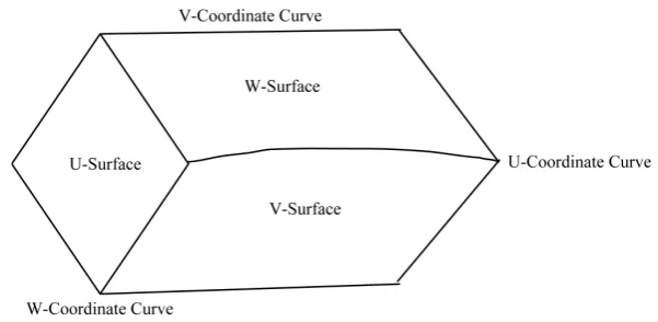
Though each point P in the given region of space, these will pass the three surfaces.

constant, constant, constant

u= v= w= (1.18)

which are known as the coordinate surfaces. Any two of these constant surfaces intersect in a space curve. The set of three curves through the point P is known as the coordinate curves of the point P. As a matter of nomen-clature, we shall adopt the following convention to distinguish between the coordinate curves:

coordinate curve, constant, constant coordinate curve, constant, constant coordinate curve, constant, constant

u v w

v w u

w u v

= = = 



= = = 



= = = _

(1.19)

The coordinate surfaces and coordinate curves associated with the point P are given in Figure 1.

If r is the radius vector from an arbitrary origin to the point P, it can be regarded as a function of a genera-lized coordinates of the point.

(

, ,

)

r =r u v w (1.20)

The change in the radius vector r due to infinitesimal displacements along the three coordinate curves is

dr rdu rdv r dw

u v w

∂ ∂ ∂

= + +

[image:7.595.162.463.82.229.2]

Figure 1. Coordinate surfaces and coordinate curve.

Thus, the change in r due to a unit displacement along the u-coordinate curve is r

u

∂

∂ . Similarly, unit

dis-placement along the v and w-coordinate curves induce the changes r

v

∂ ∂ and

r w

∂

∂ respectively. We define the set

of vectors:

1 , 2 , 3

r r r

e e e

u v w

∂ ∂ ∂

= = =

∂ ∂ ∂ (1.22)

which are known as the unitary vectors associated with the point P. It is to be noted that those vector are not generally of unit length, and that their dimensions depend on the nature of the generalized coordinates. They do, however, serve as a base of reference in the sense that any vector whose initial point is at P can be expressed as a linear combination of the set of unitary vectors.

In particular

1 2 3

dr =e ud +e vd +e wd . (1.23)

Since the set of unitary vectors are non-coplanar, they define a parallelepiped whose volume is given by

(

)

(

)

(

)

1 2 3 2 3 1 3 1 2

V = ⋅e e ×e = ⋅e e ×e = ⋅e e×e . (1.24)

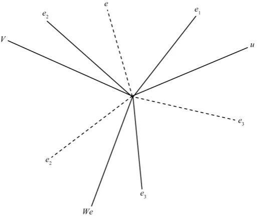
We may define triplet of vectors, known as the reciprocal unitary vectors by the relation

1 2 3 1 3 1 1 1 2

1 , 2 , 3

e e e e e e

e e e

V V V

− ₌ × − ₌ × − ₌ ×

. (1.25)

It is clear that from the definition 1

e− is normal to the plane defined by the unitary vectors (e₂, e₃). Similarly 2

e− is normal to the plane of (e₃, e₁) and 3

e− is normal to the plane of (e₁, e₂), then it follows that

1 1 1

1 2 1 3 1 1

1 1 1

2 3 2 1 2 2

1 1 1

3 1 3 2 3 3

0, 1

0, 1

0, 1

e e e e e e

e e e e e e

e e e e e e

− − −

− − −

− − −



⋅ = ⋅ = ⋅ =



⋅ = ⋅ = ⋅ = 



⋅ = ⋅ = _{⋅ = }

(1.26)

The set of nine Equations (1.26) is usually written

1 i

i j j

e− ⋅ =e

δ

(1.27)

where the symbol

δ

ij known as kroneckar delta, is defined by

1, 0,

i j

i j i j

δ

=  =_≠

 (1.28)

[image:8.595.186.443.86.304.2]

Figure 2. Relation between the unitary vectors and the reciprocal un-itary vectors.

In terms of the reciprocal unitary vectors, the differential dr has the representation:

1 1 1

1 2 3

dr =e−du′+e−dv′+e−dw′. (1.29) The differentials duʹ, dvʹ and dwʹ are obviously the components of dr in the direction specified by the reci-procal unitary vectors and are functions of the generalized coordinates (u, v, w). However, these differentials are related of the generalized coordinates by a set of linear equations which are not in general integrable. If we equate the representations of dr in terms of unitary and reciprocal unitary vectors we have:

1 1 1

1 2 3 1 2 3

dr =e ud +e vd +e wd =e−du′+e−dv′+e−dw′. (1.30)

Now we form the inner product of dr successfully with 1

e− , 2

e− and 3

e− and use the orthogonality rela-tions to obtain the set of equarela-tions:

1 1 1 1 1 1

1 1 1 2 1 3

1 1 1 1 1 1

2 1 2 2 2 3

1 1 1 1 1 1

3 1 3 2 3 3

d d d d

d d d d

d d d d

u e e u e e v e e w

v e e u e e v e e w

w e e u e e v e e w

− − − − − −

− − − − − −

− − − − − −



′ ′ ′

= + +



′ ′ ′

= + + 



′ ′ ′

= + + _

(1.31)

Similarly, if we take the inner product of dr with e₁, e₂ and e₃ we obtain the differential equations:

1 1 1 2 1 3

2 1 2 2 2 3

3 1 3 2 3 3

d d d d

d d d d

d d d d

u e e u e e v e e w v e e u e e v e e w w e e u e e v e e w

′ = ⋅ + ⋅ + ⋅ 



′ = ⋅ + ⋅ + ⋅ 



′ = ⋅ + ⋅ + ⋅ _

(1.32)

It is convenient to represent the inner product of the unitary vectors, and the reciprocal unitary vectors by the set of quantities:

1 1

ij ji

i j

ij j i ji

g e e g

g e e g

− − _

= ⋅ _



= ⋅ = _ (1.33)

11 12 13

21 22 23

31 32 33

d d d d

d d d d

d d d d

u g u g v g w

v g u g v g w

w g u g v g w



′ ′ ′

= + +



′ ′ ′

= + + _



′ ′ ′

= + + _

(1.34)

and

11 12 13

21 22 23

31 32 33

d d d d

d d d d

d d d d

u g u g v g w

v g u g v g w

w g u g v g w

′ = + + 



′ = + + _



′ = + + _

(1.35)

Now, consider and arbitrary vector a which has initial point at the point p. This vector may be repre- sented in terms of either the set of unitary or reciprocal unitary vectors:

3 3

1

1 1

i

i i i

i i

a a e a e−

= =

=

∑

=

∑

(1.36)

where ai and ai are the projections of a in the direction of ei and i

e respectively. If we form the inner product of a_i with i

e we obtain as a result of the orthogonality relations

1 i

i a = ⋅a e− similarly

i i

a = ⋅a e.

The two sets of components of the vector space a̅ are related to one another by

3 3

1 1

,

j ij i

i i ji

j i

a g a a g a

= =

=

∑

=

∑

. (1.37)

The arbitrary vector a thus has either of the representations:

(

)

(

)

3 3

1 1

1 1

i

i i i i i

i i

a a e− e a e e−

= =

=

∑

=

∑

. (1.38)

In the generalized coordinate system (u, v, w). The quantities ai are known as the contra variant components of the vector a relative to the coordinate system (u, v, w). Similarly the set of quantities ai are known as the

covariant components of the vector a relative to the coordinate system (u, v, w).

Since the lengths and dimensions of the unitary and reciprocal unitary vectors depends on the nature of the set of generalized coordinates. It is clear that the covariant and contra variant components of given vector do not necessarily have the same dimensions as the given vector. In order to avoid difficulties which may be introduced by this fact, it is frequently desirable to define a set of unit vectors, but which are dimensionless.

3 3

1 1 2 2

1 2 3

11 22 33

1 1 2 2 3 3

, , e e

e e e e

i i i

g g g

e e e e e e

= = = = = =

⋅ ⋅ ⋅ (1.39)

In terms of this set of dimensionless unit vectors, the arbitrary vectors a has the representation:

1 1 2 2 3 3

a=A i +A i +A i . (1.40)

The set of components Ai have the same dimensionality as the given vector a. These are known as the physical

components of the vector a relative to the coordinate system (u, v, w).

4.2. Line, Surface and Volume Elements

The vector dr represents a displacement from the point P(u, v, w) to the point Q u

(

+d ,u v+d ,v w+dw

)

we shall define:

2

1 1 1 2 1 3 2 1 2 2

2 3 3 1 3 2 3 3

d d d d d d d d d d d d d

d d d d d d d d

S r r e e u u e e u v e e u w e e u v e e v v e e v w e e w u e e w v e e w w

= ⋅ = + + + +

In terms of the coefficients gij, this may be written

2

11 12 13 21 22

23 31 32 33

d d d d d d d d d d d

d d d d d d d d

S g u u g u v g u w g v u g v v g v w g w u g w v g w w

= + + + +

+ + + + (1.42)

We may also express the quantity dS2 in terms of the reciprocal unitary vectors by:

2 11 12 13 21 22

23 31 32 33

d d d d d d d d d

d d d d d d d d

S g u u g u v g du dw g v u g v v

g v w g w u g w v g w w

′ ′ ′ ′ ′ ′ ′ ′ ′ ′

= + + + +

′ ′ ′ ′ ′ ′ ′ ′

+ + + + (1.43)

The gij and gij appear as the coefficients of two differential quadratic forms which express the square of the arc

length in the space of the generalized coordinates (u, v, w) or the related coordinates (uʹ, vʹ, wʹ).

Now, let dS1 represent an infinitesimal displacement along the u-coordinate curve from the point P(u, v, w). Then

1 1 1 1 11

dS =e ud , dS = dS = g du (1.44)

Similarly, the length of arc along the v-coordinate and w-coordinate curves are given by

2 22 3 33

dS = g d , dv S = g dw (1.45) respectively.

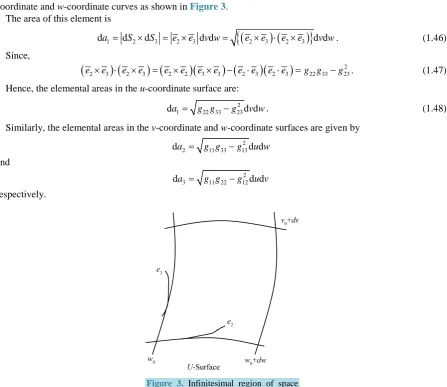
Let us consider and infinitesimal elemental of the u-coordinate surface, which is bounded by intersecting v- coordinate and w-coordinate curves as shown in Figure 3.

The area of this element is

(

) (

)

{

}

1 2 3 2 3 2 3 2 3

da = dS ×dS = e ×e d dv w= e ×e ⋅ e ×e d dv w. (1.46)

Since,

(

) (

) (

)(

) (

)(

)

2

2 3 2 3 2 2 3 3 2 3 2 3 22 33 23

e ×e ⋅ e ×e = e ×e e ×e − e e⋅ e e⋅ =g g −g . (1.47)

Hence, the elemental areas in the u-coordinate surface are:

2 1 22 33 23

da = g g −g d dv w. (1.48)

Similarly, the elemental areas in the v-coordinate and w-coordinate surfaces are given by

2 2 11 33 13 da = g g −g d du w

and

2 3 11 22 12 da = g g −g d du v

respectively.

[image:10.595.91.539.321.708.2]

The infinitesimal region of space bounded by three coordinate surfaces has a volume given by

(

)

(

)

1 2 3 1 2 3

dv=dS ⋅ ds ×dS = ⋅e e ×e d d du v w. (1.49)

It follows from Equation (1.49) that the cross product e₂×e₃ can be written as:

(

1

) (

1

) (

1

)

2 3 1 2 3 1 2 2 3 2 3 2 3 3

e × =e e e− ×e e + e e− ×e e + e e− ×e e . (1.50)

It follows from the definition of the reciprocal unitary vectors that we can rewrite equation (1.50) in the form:

(

) (

)

(

) (

)

(

) (

)

1

1 2 3 2 3 1 2 1 3 1 2 3 2 1 2 3 1 3

1 2 3

e

e e e e e e e e e e e e e e e e e e

e e e

−

 

⋅ × = _ × ⋅ × + × ⋅ × + × ⋅ × _

×

which is equivalent to

(

)

(

) (

) (

) (

)

(

) (

)

(

) (

)

(

) (

) (

) (

)

(

)

(

)

(

)

2

1 2 3 1 1 2 2 3 3 2 3 3 2 1 2 2 3 3 1

2 1 3 3 1 3 2 1 3 2 2 2 3 1

11 22 33 23 32 22 23 31 21 33 33 21 32 22 31

e e e e e e e e e e e e e e e e e e e

e e e e e e e e e e e e e e

g g g g g g g g g g g g g g g

  

⋅ × = ⋅ _ ⋅ ⋅ ⋅ − ⋅ ⋅ ⋅ _+ ⋅ _ ⋅ ⋅ ⋅

  

− ⋅ ⋅ ⋅ _+ ⋅ _ ⋅ ⋅ ⋅ − ⋅ ⋅ ⋅ _

= − + − + −

(1.51)

The right hand side of Equation (1.51) is the expansion of the determinant

11 12 13

21 22 23

31 32 33

g g g

g g g g

g g g

= (1.52)

Hence the increment volume is expressed in terms of the generalized coordinates (u, v, w) by:

dV = g u v wd d d . (1.53)

For the sake of simplicity, it will be convenient to make certain changes in notations and to introduce the so called Einstein summation convention. The change in notation which we require is the following:

1 2 3

1 2 3

, ,

, ,

u u v u w u

x x y x z x

= = =

= = = (1.54)

The summation convention which we shall adopt is the following. Whenever a Latin index appears both as a subscript and a superscript is the same expression, it is summed from 1 to 3. For example:

1 2 3

1 2 3

d d d d

ij i i i i

g =g u +g u +g u = u . (1.55)

In order to complete the convention, we shall adopt the rule that whenever an index appears as a subscript in the denominator of a fraction, it is regarded as equivalent to superscript in the numerator for purpose of summation and vice versa. For example:

1 2 3

1 2 3

k

k

u u u u

x x x x

∂ ₌∂ ₊∂ ₊∂

∂ ∂ ∂ ∂ (1.56)

4.3. The Differential Operators in Generalized Coordinates

The gradient of a scalar function ρ(u1, u2, u3) is a fixed vector which is defined to have the direction and magnitude of the maximum rate of change of ρ with respect to the coordinates. The variation in ρ corresponding to the infi-nitesimal displacement dr is

d dr grad _i dui u

ρ

ρ

= ⋅

ρ

= ∂

∂ . (1.57)

Now the dui are the contra variant components of the infinitesimal displacement dr, and hence; 1

dui dr ei

−

= ⋅ . (1.58)

1

2 i d 0

grad e r

u

ρ

ρ ∂ −

 ₋  ₌

 _∂ 

  . (1.59)

Since the displacement dr is arbitrary, it follows that the bracketed term in (1.59) must vanish identically. Thus the representation of gradient of the scalar field in terms of the generalized coordinates (u1, u2, u3) is

1

i i

grad e

u

ρ

ρ

₌ ∂ −

∂ . (1.60)

The representation (1.60) is in terms of reciprocal unitary vectors, and hence, the quantities _i

u

ρ ∂

∂ represent

the covariant components of the gradient ρ. We may obtain a representation in terms of the unitary vectors from the relations:

1 ij 1

i j

e− =g e− . (1.61)

If we substitute these relations in (1.60), we obtain the representation

ij i

grad g u

ρ

ρ

= ∂

∂ . (1.62)

We then identify the contra variant components of gradρ as

(

)

i ij

j

grad g

u

ρ

ρ

= ∂

∂ . (1.63)

The representation of the divergence of the vector field

(

1 2 3

)

, ,

a u u u in terms of the generalized coordinates is easily obtained from the definition:

(

1 2 3

)

0

dd , , lim s

v

a n s diva u u u

v

∇ ∇ →

⋅ =

∇

∫

. (1.64)

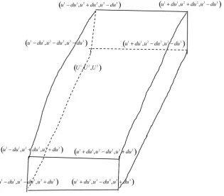
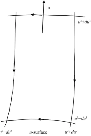
[image:12.595.160.476.427.703.2]

We shall evaluate the surface integral over the surface bounding the volume shown in Figure 4.

Figure 4. Surface bounding the volume

(

1 2 3

)

The volume is bounded by the coordinate surface u1−du1, u1+du1, u2−du2, u2+du2, u3−du3, u3+du3

we consider the contribution to the surface integral from the two ends of the volume element which lie in u1-surface. At the face u1+du1 we have:

(

)

2 2

2 2

dd 4 d d

n s= e ×e u u , while at the face 1 1 d

u − u , ndds=4

(

e₃×e₂

)

du2du3.

The contribution to the surface integral from these two faces is

(

)

1 1

(

)

1 1

2 3 3 2

2 3 _d 3 2 _d

4 d d 4 d d

u u u u

a e e u u ₊ a e e u u ₋

 ⋅ ×  +  ⋅ × 

   

where the subscript indicates that the quality in brackets is to be evaluated at the point indicated. The contribution to the surface integral from these two faces can be shown to be

( )

1 2 3

1

8 a g d du u du u

∂

∂ . (1.65)

These are analogous contributions from the remaining two pairs of faces. Adding, all the contributions to the surface integral dividing by

1 2 3

dv=8 g u ud d du

and going to the limit du1→ 0, du2→ 0 we obtain the desired representation

( )

1

i

diva a g

u g

∂ =

∂ . (1.66)

The representation of the curl of a vector field in terms of the set of generalized coordinates (u1, u2, u3) is also easily obtained from the definition

0 d lim c

s

a e n curla

s

∆ →

⋅

⋅ =

∆

∫

(1.67)

where Cis a closed contour bounding the surface ∆S, which has unit positive normal n. We shall evaluate the live integral about the contour. This bounds a rectangular region in the u1-coordinate surface as in Figure 5 the di-rection of the contour has been chosen, so that the positive normal is in the didi-rection of the position u1-coordinate curve. The contribution to the live integral from the sides which are parallel to the u2-coordinate curve is

[image:13.595.238.391.469.696.2]

(

)

3 3

(

)

3 3

2 2

2 2

d d

d d

u u u u

a e u a e u

+ −

   

−_ ⋅ _ +_ ⋅ _ . (1.68)

Similarly the sides parallel to the u3-coordinate curves provide a contribution

(

)

2 2

(

)

2 2

3 3

3 d _{u du} 3 d _{u du}

a e u a e u

+ −

   

−_ ⋅ _ +_ ⋅ _ . (1.69)

Approximating Equations (1.68) and (1.69) by the linear terms of their Taylor series we find that the line integral is approximately by

(

)

(

)

2 3

3 2

2 3

4 a e a e d du u

u u

∂ ∂

 _{⋅ − ⋅} 

_{∂ ∂} 

  . (1.70)

This quantity must now be divided by the area of the rectangular region which is

(

) (

)

{

}

2 3

2 3 2 3

4 d d

S e e e e u u

∆ = × ⋅ × . (1.71)

The reciprocal unitary vectors 1

e− is always orthogonal to the u1-coordinate surface, so that the unit must normal to the open surface is

{

}

1

1 1

e n

e e

− − −

=

⋅ (1.72)

then

(

)

(

)

{

}

{

(

) (

)

}

(

)

(

)

1

3 2

2 3

1 1

2 3 2 3

1 e

curla n curla a e a e

u u

e e e e

e e

− − −

∂ ∂

 

= = _ ⋅ − ⋅ _

∂ ∂

 

× ⋅ ×

⋅ (1.73)

which will easily change to:

3 2 1 3 2 1

1 2 3

2 3 3 1 1 2

1 a a a a a a

curla e e e

u u u u u u

g

 ∂ ∂  ∂ ∂  ∂ ∂  

= _ − _ +_ − _ +_ − _{ }

∂ ∂ ∂ ∂ ∂ ∂ 

   

 . (1.74)

Equation (1.74) is the contra variant representation of curl a with respect to the generalized coordinate system (u1, u2, u3).

5. Orthogonal Coordinate System

An orthogonal system is defined by the requirement that the unitary vectors (e1, e2, e3) are everywhere mutually orthogonal

1

i j ij ij

e− ⋅ =e e

δ

. (1.75)

Under these conditions, the reciprocal unitary vector e−i is parallel to e_i and is given by

1 1 1

i i i

i j ij

e e e

e e g

− _{= ⋅ =}

. (1.76)

It follows from Equation (1.76) that the metric coefficients gij vanish whenever i≠ j. For orthogonal

coor-dinate system, it is necessary to define a set of scalar factors:

i ij

h = g . (1.77)

In the case of an orthogonal system the set of second metric coefficients are given by:

2

1 1

ij

ij ij i

g

g h δ

= = (1.78)

from the sum of the first metric coefficients it follows that the scalar factors are calculated by

2 2 2

1 2 3

2

i i i i

x x x

h

u u u

∂  ∂  ∂ 

=_{ } +_{ } +_{ }

∂ ∂ ∂

The element cell which is bounded by the coordinate surfaces is the rectangular region bounded by the edge of length

1 2 3

1 1 2 2 3 3

dS =h ud , dS =h ud , dS =h ud .

The volume of this elementary cell is

1 2 3

1 2 3

dv=h h h u ud d du . (1.80)

It is easy to see that thus is a special case of the previous result for the elementary volume ion a generalized coordinate system,

1 2 3

dv= g u ud d du .

In the case of an orthogonal system, all of the off diagonal terms in det(gij) are zero, and consequently

2 2 2 1 2 3 g=h h h .

In a fixed coordinate system the advantages of using either covariant or contra variant components of a given vector a, in terms of its physical components relative to the orthogonal unit base

(

i i i₁, ,_{2 3}

)

where

1 , i

i i i i

i

e h i e i

h

= = .

For an orthogonal system, we have the relatively simple relations between the covariant, contra variant and physical components of the vectors a,

1 ,

i i

i i i

i

a A a h A

h

= = .

The differential operator relative to an orthogonal curvilinear coordinate system can be immediately deduced as special cases of the general results. It follows from Equation (1.62) that in an orthogonal system, the gradient of a scalar field has the representation:

3

1 1

j

j j

grad ij

h u

φ φ

=

∂ =

∂

∑

. (1.81)

The divergence of a vector field in terms of an orthogonal curvilinear system can be obtained as special case of Equation (1.66).

(

2 3 1

)

(

3 1 2

)

(

1 2 3

)

1 2 3

1 2 3 1

diva h h A h h A h h A

h h h u u u

∂ ∂ ∂

 

= _ + + _

∂ ∂ ∂

  (1.82)

Similarly, it follows from Equation (1.74) that is an orthogonal curvilinear system, the curl of a vector field has the representation

(

)

(

)

(

)

(

)

(

)

(

)

3 3 2 2 1

1 3

2 3

3 3 3 3 2

3 1

3 1

2 2 1 1 3

1 2

1 2 1

1

1

curla h A h A i

h h u u

h A h A i

h h u u

h A h A i

h h u u

∂ ∂

 

= _ − _

∂ ∂

 

∂ ∂

 

+ _ − _

∂ ∂

 

∂ ∂

 

+ _ − _

∂ ∂

 

(1.83)

In Equation (1.82) and (1.83), the quantities Ai are the physical components of the vector a̅ relative to the

coordinate system (u1, u2, u3). We note that Equation (1.83) is the normal expansion of the determinant.

1 1 2 2 3 3

1 2 3

1 2 3

1 1 2 2 3 3 1

h i h i h i

curla

h h h u u u

h A h A h A

∂ ∂ ∂

=

6. Some Vector Relations in Curvilinear Coordinates

In this section, we shall list the basic vector relations for two important curvilinear coordinate systems. We shall use the notation (u, v, w) for the curvilinear systems, with the exception that in systems with cylinder symmetry, the coordinate axis along the symmetry axis will be denoted by z. The unit vector associated with the coordinate systems is specified in terms of their Cartesian representation, and all vector results are given in terms of physical components.

6.1. Parabolic Cylindrical Coordinates

(

)

2 , ,

x= u v− y= uv z=Z

0≤ < ∞ ≤ < ∞ −∞ < < ∞u , 0 v , z

1 2 3

1 1

, , 1

2 2

u v u v

h h h

u v

+ +

= = =

The constant coordinate surfaces are:

2 2

2 2

constant parabolic cylinders 2

constant parabolic cylinders 2

constant planes normal to the cylinder axis

u Y ux u

v Y vx v

z

= − + =

= − − =

= −

(1.85)

The unit vectors are

1

2

3

u v

i i j

u v u v

v u

i i j

u v u v

i k



= + _

+ + _



= − ₊ + ₊ 

  =

 

(1.86)

1 2 3

2

grad u i v i i

u v z

u v

φ φ φ

φ= _ ∂ + ∂ _+∂

∂ ∂ ∂

+   (1.87)

(

)

(

)

(

(

)

)

3

1 2

2 A

divA u u v A v u v A

u v u v z

∂

∂ ∂

 

= _ + + + _+

+  ∂ ∂  ∂ (1.88)

(

)

(

)

(

(

)

)

3 2 1 3

1 2

2 1 3

1

2 2

2

A A A A

curlA v u v i u v u i

v z z u

u v

u u v A v u v A i

u v u v

 _{∂ ∂}  _{ ∂ ∂ } 

 

= ₊ _{ ∂} − + _{∂ } +_ + _∂ − _∂ _ 

  

 

∂ ∂

 

+ _ + − + _

+  ∂ ∂ 

(1.89)

2 2

2 4

u u v v

u v u u v v z

φ

φ

φ

φ

 ∂  ∂  ∂  ∂  ∂

∇ = _{  }+ _{ }+

+  ∂  ∂  ∂  ∂  ∂ (1.90)

6.2. Ellipsoidal Coordinates

(

)(

)(

)

(

)(

)

2 2 2

2 2 2 2

a u a v a w

x

a b a c

 − − − 

 

=  

− −

 

(

)(

)(

)

(

)(

)

2 2 2

2 2 2 2

b u b v b w

y

b a c b

 − − −    =   − −    

(

)(

)(

)

(

)(

)

2 2 2

2 2 2 2

c u c v c w

z

a c b c

 − − −    =   − −    

2 2 2

u c v b w a

−∞ < ≤ ≤ ≤ ≤ ≤

(

)(

)

(

)(

)(

)

1 _{2 2 2}

1 2

v u w u h

a u b u c u

 _{− −}    = _{ } − − −    

(

)(

)

(

)(

)(

)

2 _{2 2 2}

1 2

u v w v h

a v b v c v

 _{− −}    = _{ } − − −    

(

)(

)

(

)(

)(

)

3 _{2 2 2}

1 2

u w v w h

a w b w c w

 _{− −}    =   − − −    

The constant coordinate surfaces are

2 2 2

2 2 2

2 2 2

2 2 2

2 2 2

2 2 2

constant ellipsoids 1

constant hyperboloids of one sheet 1

constant hyperboloids of two sheet 1

x y z

u

a u b u c u

x y z

v

a v b v c v

x y z

w

a w b w c w

= − + + = − − − = − + + = − − − = − + + = − − − (1.91)

The unit vectors are:

(

)(

)(

)(

)

(

)(

)

(

)(

)

(

)(

)(

)(

)

(

)(

)

(

)(

)

(

)(

)(

)(

)

(

)(

)

(

)(

)

2 2 2 2

1 _{2 2 2 2}

2 2 2 2

2 2 2 2

2 2 2 2

2 2 2 2

b u c u a v a w

i i

v u w u a b a c

a u c u b v b w

j

v u w u b c a b

a u b u c v c w

k

v u w u a c b c

 − − − −    =   − − − −      − − − −    +   − − − −      _{− − − −}    +   − − − −    

(

)(

)(

)(

)

(

)(

)

(

)(

)

(

)(

)(

)(

)

(

)(

)

(

)(

)

(

)(

)(

)(

)

(

)(

)

(

)(

)

2 2 2 2

2 2 2 2 2

2 2 2 2

2 2 2 2

2 2 2 2

2 2 2 2

b v c v a u a w

i i

u v w v a b a c

a v c v b u b w

j

u v w v b c a b

a v b v c u c w

k

u v w v a c b c

(

)(

)(

)(

)

(

)(

)

(

)(

)

(

)(

)(

)(

)

(

)(

)

(

)(

)

(

)(

)(

)(

)

(

)(

)

(

)(

)

2 2 2 2

3 _{2 2 2 2}

2 2 2 2

2 2 2 2

2 2 2 2

2 2 2 2

b w c w a u a v

i i

u w v w a b a c

a w c w b u b v

j

u w v w b c a b

a w b w c u c v

k

u w v w a c b c

 _{− − − −}    =   − − − −      − − − −    +   − − − −      _{− − − −}    +   − − − −     (1.92)

(

)(

)(

)

{

}

(

)(

)

(

)(

)(

)

{

}

(

)(

)

(

)(

)(

)

{

}

(

)(

)

2 2 2

1

2 2 2

2

2 2 2

3 2

2

2

a u b u c u

grad i

v u w u u

a v b v c v

i

u v v w v

a w b w c w

i

u w v w w

φ φ φ φ − − − _∂ = − − ∂ − − − _∂ + − − ∂ − − − _∂ + − − ∂ (1.93)

(

)(

)(

)

{

}

(

)(

)

{

(

)(

)

}

(

)(

)(

)

{

}

(

)(

)

{

(

)(

)

}

(

)(

)(

)

{

}

(

)(

)

{

(

)(

)

}

2 2 2

1

2 2 2

2

2 2 2

3 2

2

2

a u b u c u

divA v u u w A

v u w u u

a v b v c v

v u w v A

v u v w v

a w b w c w

w v u w A

v w w u w

− − − _{∂ }  = _ − − _   − − ∂ − − − _{∂ }  + _ − − _   − − ∂ − − − _{∂ }  + _ − − _ − − ∂ (1.94)

(

)(

)(

)

₍

₎

(

)(

)(

)

₍

₎

(

)(

)(

)

₍

₎

(

)(

)(

)

₍

₎

(

)(

)(

)

2 2 2

3

2 2 2

2 1

2 2 2

1

2 2 2

3 2

2 2 2

2

2

2

a v b v c v

curlA v w A

v w v u v

a w b w c w

w v A i

w u w

a w b w c w

w u A

w u w v w

a u b u c u

u w A i

u v u

a u b u c u

u v v w

 − − −  _∂   _{ } = ₋  ₋ _{∂ } − _      _{− − −}  _∂   _{ } − _{  } − _ − ∂      − − −  _∂   _{ } + _{  } − _ − _ − _∂  − − −  _∂   _{ } −  ₋ _{∂ } − _      _{− − −}  _∂   + _{ } − _ − _

(

)

(

)(

)(

)

₍

₎

2

2 2 2

1 3

u v A

u

a v b v c v

v u A i

v w v