Origin of exon skipping rich transcriptomes in animals driven by evolution of gene architecture

R E S E A R C H

Open Access

Origin of exon skipping-rich transcriptomes

in animals driven by evolution of gene

architecture

Xavier Grau-Bové

, Iñaki Ruiz-Trillo

and Manuel Irimia

Abstract

Background:Alternative splicing, particularly through intron retention and exon skipping, is a major layer of pre-translational regulation in eukaryotes. While intron retention is believed to be the most prevalent mode across non-animal eukaryotes, animals have unusually high rates of exon skipping. However, when and how this high prevalence of exon skipping evolved is unknown. Since exon skipping can greatly expand proteomes, answering these questions sheds light on the evolution of higher organismal complexity in metazoans.

Results:We used RNA-seq data to quantify exon skipping and intron retention frequencies across 65 eukaryotic species, with particular focus on early branching animals and unicellular holozoans. We found that only bilaterians have significantly increased their exon skipping frequencies compared to all other eukaryotic groups. Unlike in other eukaryotes, however, exon skipping in nearly all animals, including non-bilaterians, is strongly enriched for frame-preserving sequences, suggesting that exon skipping involvement in proteome expansion predated the increase in frequency. We also identified architectural features consistently associated with higher exon skipping rates within all studied eukaryotic genomes. Remarkably, these architectures became more prevalent during animal evolution, indicating co-evolution between genome architectures and exon skipping frequencies.

Conclusion:We suggest that the increase of exon skipping rates in animals followed a two-step process. First, exon skipping in early animals became enriched for frame-preserving events. Second, bilaterian ancestors dramatically increased their exon skipping frequencies, likely driven by the interplay between a shift in their genome architectures towards more exon definition and recruitment of frame-preserving exon skipping events to functionally diversify their cell-specific proteomes.

Keywords: Alternative splicing, Exon skipping, Intron retention, Ancestral reconstruction, Gene architecture, Evolution of transcriptome regulation

Background

Alternative splicing (AS) is a pre-translational process that allows the creation of multiple messenger RNA (mRNA) transcripts from a single gene by differentially selecting splice sites in multi-exonic sequences [1]. This phenomenon can contribute to the regulation of gene expression [2–7], or the creation of multiple protein iso-forms per gene, increasing the proteomic repertoire of

eukaryotic genomes [8, 9] and potentially leading to key evolutionary innovations [10–12].

The main forms of AS among eukaryotes are the exclusion of specific exons and the retention of introns in the final transcripts [1, 13], referred to as exon skip-ping (ES) and intron retention (IR), respectively. These sources of transcript variation are widespread in eukary-otes, but initial studies revealed that the prevalence of each AS mode varied across lineages: animals show higher rates of ES than other eukaryotes, whereas IR is frequent across all eukaryotic groups, including animals, fungi, plants, and various protist lineages [14–17]. This contrast led to the proposition that ES-rich AS profiles were a major contributor to the increased phenotypic

* Correspondence:[email protected];[email protected]

1

Institut de Biologia Evolutiva (CSIC-Universitat Pompeu Fabra), Passeig Marítim de la Barceloneta 37-49, 08003 Barcelona, Catalonia, Spain

4_{Centre de Regulació Genòmica, Barcelona Institute of Science and}

Technology, Dr. Aiguader 88, 08003 Barcelona, Catalonia, Spain Full list of author information is available at the end of the article

complexity of animals, since richer proteomes can provide an expanded tool-kit needed to sustain multicellularity [8, 18]. Consistently, and although the extent to which ES transcripts are translated and functional is still under debate [19, 20], many ES-derived isoforms have been found to be physiologically relevant in animals (reviewed in [8, 21]), for example, by tuning protein–protein inter-action networks [22–24]. In contrast, IR events have been linked to down-regulation of gene expression via the nonsense-mediated decay (NMD) pathway [4–6, 25], nuclear retention [7] or intron detention [3] in a wide variety of eukaryotes.

The evolutionary origin of AS can be tracked to the last eukaryotic common ancestor (LECA), which already had an intron-dense genome [26, 27] with heterogeneous splice sites [28–30] and all the essen-tial splicing machinery (the spliceosome, a complex of small nuclear RNAs and dozens of assisting protein factors) [27, 31, 32]. These observations have allowed inferring that the earliest eukaryotes already exhibited splicing-rich transcriptomes yielding multiple mRNA variants per gene, mostly by IR [18, 33, 34]. However, it remains unclear when and how animal transcrip-tomes shifted towards higher frequencies of ES and recruited this mode of AS as a mechanism to expand their proteomes. First, the sampling of early-branch-ing species—poriferans, cnidarians, placozoans, and ctenophores—is scarce. Second, no comprehensive comparative study using high-throughput RNA se-quencing (RNA-seq) data has been performed to date. Third, relative increases in ES frequency have also been identified in other phylogenetically scattered eu-karyotes—e.g. in plants,Volvox carteri, or the chlorar-achniophyte Bigelowiella natans [10, 35–38].

Here, we address these questions by analyzing RNA-seq-derived AS profiles for 65 eukaryotic species. Using this comprehensive dataset of joint transcriptomic and genomic data, we track the frequency of both main modes of AS (IR and ES) across all major eukaryotic lineages (Fig.1a, Additional file1: Figure S1), uncovering the phylogenetic patterns behind AS evolution. Specific-ally, we investigate the transition towards high ES fre-quencies in multicellular lineages (animals and plants) by comparing their AS profiles and genome architec-tures with their closest unicellular relatives. We find that the frequency of ES rose mainly in bilaterians, with only mild increases in non-bilaterians. However, we show that recruitment of ES for proteome expansion predated the bilaterian increase in ES and occurred early in metazoan evolution. Furthermore, we uncover a set of sequence and architectural features that influence the frequency of ES and IR in transcripts across eukaryotes, suggesting the existence of a soft pan-eukaryoticcis- regu-latory code for AS determination. Using this code and reconstruction of ancestral intron–exon architectures we evaluated the step-wise increase of ES along animal evolution.

Results

ES frequency increased largely in bilaterian ancestors

We quantified the frequencies of ES and IR at the single exon and intron levels for 65 eukaryotic species (Fig.1a), including a wide range of intron–exon architectures (Fig.1b, c; Additional file 1: Figures S1 and S2). For this purpose, we compiled a large dataset of available RNA-seq data (Additional file1: Figure S1) and performed de novo RNA-seq for three phylogenetically key species: the pla-cozoanTrichoplax adhaerens, the holozoanSphaeroforma

aTaxon sampling

Excavata (1) Other Bilateria (8)

Porifera (3) Placozoa (1)

Embryophyta (6) Fungi (12)

Cryptophyta (1)

Rhizaria (1) Amoebozoa (3) Charophyta (1) Chlorophyta (3)

Fonticula(1)

Alveolata (2) Filasterea (1)

Haptophyta (1) Ichthyosporea (3)

Stramenopila (3) Cnidaria (3) Ctenophora (1) Choanoflagellata (1)

Glaucophyta (1) Metazoa

Holozoa

Viridiplantae Opisthokonta

Vertebrata (7)

Amorphea

'Bikonta' Diaphoratickes

Choanozoa

b Intron length distribution cExon length distribution

0 1 2 3 4 5 6 7

0

500

1000

1500

Introns/CDS kbp

Exon length (bp)

0 1 2 3 4 5 6 7

0

1

000

2000

3000

4000

Introns/CDS kbp

Intron length

(bp)

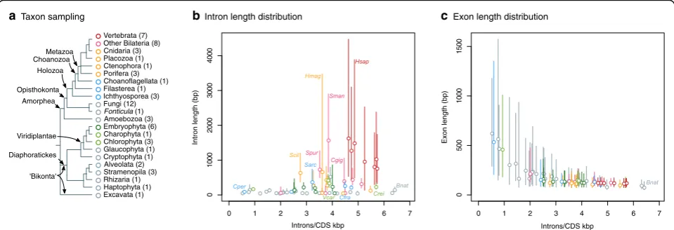
Fig. 1Intron/exon structure across eukaryotes.aSummary of the taxon sampling used in this study and the phylogenetic relationships between

species (Additional file1: Figure S1).b, cComparison of intron density (introns/CDS kbp) and intron (b) and exon (c) length distribution (in bp) in

65 eukaryotic genomes.Dotsrepresent median intron/exon lengths andvertical linesdelimit the first and third quartiles (Additional file1: Figure S2).

arctica, and the intron-rich excavate Naegleria gruberi. For the analysis of ES events (Additional file1: Figure S3), we compiled a dataset of exon triplets from 2.93 × 106 internal exons from 5.08 × 105 multi-exonic genes with transcriptomic support. Each internal exon was classified as ES-negative (0–10% exon skipping rate [rES] and sufficient read coverage; 89.29% of the dataset), ES-positive (rES= 10– 90% and sufficient read coverage; 0.74% of the data), or un-determined (all other cases; Additional file 1: Figure S4). For the analysis of IR (Additional file 1: Figure S3), an analogous dataset was built with 1.98 × 106introns from 3.88 × 105 multi-exonic genes, which were classified as IR-negative (0–10% inclusion rate [rIR] and sufficient read coverage; 71.09% of the data), IR-positive (rIR= 10–90%, and sufficient read coverage; 5.27% of the data), or un-determined (Additional file1: Figure S4).

Next, we examined the frequency of each AS mode at the species level by averaging exon- and intron-specific ES and IR rates across 100 subsets of exons or introns with normalized RNA-seq coverage (FES,sp and FIR,sp, respectively; see “Methods”; Additional file1: Figures S3 and S5). This analysis produced three major results. First, we found evidence of ES and IR in transcriptomes from all studied eukaryotic lineages—namely, animals, fungi, opisthokont protists, amoebozoans, Viridiplantae, the cryptophyte Guillardia theta, SAR, the haptophyte Emiliania huxleyi, and the excavate Naegleria gruberi (Fig. 2, Additional file 1: Figures S4 and S6). Second, IR frequencies exceeded ES in all but one species (Fig. 2b). This result is in line with previous reports highlighting the dominance of IR-based AS across eukaryotes, but challenges initial views of animal transcriptomes as being dominated by ES. A possible explanation for this disagreement is the association between high IR rates and low transcript expression levels (see below), which hinders the detection of retained introns (particularly in studies based on EST data [14,15,39]).

Third, we found a clear phylogenetic pattern behind ES frequencies (Fig. 2a): animals, particularly bilaterians, had the highest frequencies, followed by non-bilaterians, plants, and a handful of other scattered eukaryotes. The consistency of our quantifications at the species level was assessed with replicate transcriptomic datasets for six selected ES-rich taxa obtained from independent studies (Additional file 1: Figure S7). Species-level FES,sp values were highly consistent between pairs of multi-organ tran-scriptomic datasets of adult human, frog, and tale cress and a comparison of developmental time series with various growth conditions for fruit fly (p > 0.01, Wilcoxon rank-sum test). Mild significant differences were observed between two multi-organ sets of mouse (p = 0.0037, Wilcoxon rank-sum test) and a comparison of devel-opmental series of the sea anemone Nematostella vectensis (p = 1.67e−08, Wilcoxon rank-sum test), but

in both cases the distributions were within their re-spective taxonomic ranges. Similarly, although pooled samples generally had higher ES levels than the indi-vidual tissues, the latter also fell within the taxonomic range (Additional file1: Figure S8). This indicates that our approach for ES quantification yields robust results independently of the experimental approaches used in different RNA-seq experiments.

To further investigate when the shift towards ES-rich transcriptomes occurred in animal evolution, we next compared the aggregated ES frequencies of vertebrates, non-vertebrate bilaterians, non-bilaterians (cnidarians, poriferans, the ctenophore Mnemiopsis leidyi, and the placozoan Trichoplax adhaerens), and their closest unicellular relatives in the Holozoa (choanoflagellates, Capsaspora owczarzaki, and ichthyosporeans) (Fig.2c–f; complete report of statistical comparisons in Additional file1: Figure S9).

Taken together, bilaterian animals have significantly higher FES,sp than non-bilaterians, unicellular holozo-ans, and other opisthokonts (Fig. 2c; p< 1.0e−76 in all comparisons, one-sided Kolmogorov-Smirnov test [oKS]). Furthermore, vertebrates exhibited an enrich-ment compared to other bilaterians (p = 1.0e−03). The grouping of non-bilaterians did not show signifi-cantly higherFES,spthan unicellular holozoans (Fig.2c), although different patterns were observed when com-paring against individual groups (Fig. 2d): FES,sp values were higher in cnidarians and the ctenophore M. leidyi and lower in poriferans and T. adhaerens. On the other hand, the ichthyosporean Sphaeroforma arctica had the highest FES,sp among unicellular holozoans (Fig. 2e;

p< 1e−09, oKS), which indicates a clear lineage-spe-cific departure from the low incidence of ES in other unicellular holozoans [40, 41]. Importantly, these patterns were robust to different levels of read depth downsampling across species (Additional file 1: Figure S10). Therefore, these data show that (i) bilater-ians, and vertebrates in particular, have a consistently higher ES frequency than their close relatives and other eukaryotes, and (ii) some non-bilaterian animals and unicellular holozoans have experienced relative increases in ES frequency as well.

In parallel, multicellular land plants also exhibited higher ES rates than other ‘bikonts’ (Dipahoratickes andN. gru-beri), including their colonial and unicellular relatives in Chlorophyta and Charophyta (Fig. 2f; all p< 1.0e−06, oKS). However, the colonial chlorophyte Volvox carteri was a notable exception, with higherFES,spthan other algae (including its close unicellular relative Chlamydomonas reinhardtii[38]) and most land plants (p< 1e−13 for all comparisons, oKS).

The analysis of two recent transcriptomic datasets [42, 43] showed significantly lower ES frequencies than those reported in the original genome paper [36] (Additional file 1: Figure S7; p < 1e−16, Wilcoxon rank-sum test). The reasons behind these differences remain elusive. One possible explanation is that they were caused by differences in environmental condi-tions, such as abiotic stress, which have been shown to lead to increased levels of both spurious ES and IR in other species [44–46].

Enrichment in frame-preserving ES is common to all animal groups

Next, we examined the potential global impact of AS events on each species’ proteome by assessing their ef-fect on the coding capacity of the resulting transcripts. Following previous studies [47], we divided exons or introns between those that had lengths divisible by three (henceforth ‘3n’) and those that did not, under the assumption that 3n sequences would not normally dis-rupt the open reading frame (ORF) integrity when

a c

d

e

f b

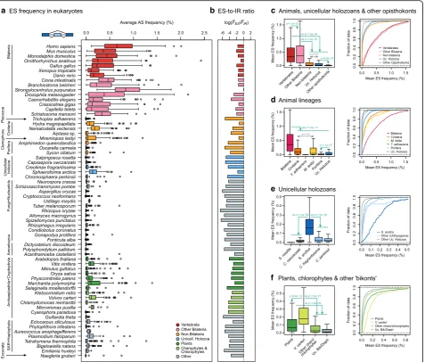
Fig. 2Frequency of AS in eukaryotes.aDistribution of ES frequencies across 65 eukaryotic transcriptomes. Each box plot represents the

distribution of ES frequencies (FES,sp) in a given species (as percentage), drawn from mapping up to 10,000 RNA-seq reads to junctions from 100

exon triplets, in up to 100 independent subsets (see“Methods”and Additional file1: Figure S3).bLog-ratio of meanFES,sp(for ES) over meanFIR,sp

(for IR) in each species.FIR,spdistributions in Additional file1: Figure S6.c–fComparisons of ES frequencies among phylogenetically related

eukaryotic groups with a focus on animals, holozoans, and plants. Group-level ES distributions obtained by poolingFES,spof multiple species. For

each set of comparisons, we report the pooled distributions’box plots (left) and empirical cumulative distributions (right). Selectedpvalues are

reported, corresponding to pairwise one-sided Kolmogorov-Smirnov two-sample tests (full report in Additional file1: Figure S9), and should be

interpreted as follows:green arrowsindicate that the group of origin has significantly higherFES,spthan others;grey bidirectional arrowsindicate

alternatively spliced, whereas non-3n sequence lengths would cause frame-shifts, usually resulting in unproduct-ive transcripts. Indeed, maintenance of the ORF integrity is strongly associated with functional and conserved ES events in animals [8,47,48].

In the case of IR, virtually no significant biases towards or against 3n divisibility were observed (Fig.3a and Additional file1: Figure S11). In contrast, we found that alternatively spliced exons of most animals were significantly enriched in 3n divisible lengths (Fig. 3b, Additional file 1: Figure S12; p< 0.01, Fisher’s exact test). This includes all vertebrates, most bilaterians, the ctenophore M. leidyi, and the cnidarians Aiptasia sp. and H. magnipapillata (p < 0.05). For example, 37.8% of M. leidyi’s ES-negative exons were 3n divisible, but this percentage increased up to 76.9% in ES-positive exons. Overall, the fraction of 3n divisible exons was

higher in ES-positive exons than in ES-negative ones for 20 out of 23 animal species, and at least half of the ES-positive exons were 3n divisible in 15 out of 23 animals (Fig.3c), suggesting that exon 3n enrichment is largely an animal feature. This enrichment was also observed when individual, rather than pooled, tissues were analyzed (Additional file 1: Figure S13A) and at different levels of sequencing depth (Additional file 1: Figure S14). Moreover, this pattern was even stronger when we restricted the analysis to highly alternative exons (rES = 30–70%; Fig. 3d). Most animals showed higher 3n enrichment in this subset, including robust increases in some non-bilaterians that did not exhibit significant 3n biases in the whole transcriptome. For example, the 3n fraction of ES-negative exons of the sponge Amphimedon queenslandica is 43.2%, but in-creases to 73.1% in highly alternative ES-positive ones

a b c

e d

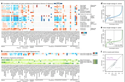
Fig. 3Fraction of 3n divisible exon and intron lengths.aPercentage of introns with 3n divisible lengths that were classified as IR-negative (x-axis)

and IR-positive (y-axis) in each species with more than ten IR-positive introns.bPercentage of exons with 3n divisible lengths that were classified

as ES-negative (x-axis) and ES-positive (y-axis) in each species with more than ten ES-positive exons.Dotsare color-coded according to enrichments in

either direction (3n bias inblue, anti-3n bias inred) as per Fisher’s exact test (p< 0.01; Additional file1: Figure S9).cPercentage of ES-positive exons

that are 3n (y-axis) with respect to the percentage of genes with ES-positive exons (x-axis), per species. Shading colors grouping the most

representative species for certain eukaryotic groups (bilaterians, non-bilaterians, and other eukaryotes) are provided for reference.dFraction of 3n

exons in ES events (rES= 10–90%,grey bar segment) compared to a subset of high-frequency events (rES= 30–70%), highlighting increases (blue) or

decreases (red) of the 3n fraction. In panelsdande, asterisks indicate significant 3n biases in ES-positive compared to ES-negative exons, as per

Fisher’s exact test (p< 0.01; Additional file1: Figure S9). In all panels, only species with more than ten exons in all categories are included.eFraction of

3n exons in ES events (grey bar segment) compared to a subset of genes with above-median expression (cRPKM) and gene length (‘high constraint’),

(p = 2.55e−3, Fisher’s exact test), and a mild increase also occurs in another sponge,Sycon ciliatum (p= 0.022; Fisher’s exact test; Additional file1: Figure S12).

On the other hand, lack of positive 3n biases was ob-served in nearly all other eukaryotes, including unicellular holozoans and plants, reaching negative enrichments (S. arcticaand the plantsVitis viniferaandPhyscomitrella patens) and/or reducing this enrichment in the highly alternative subset in some species (Oryza sativa and P. patens) (Fig.3b–d). Only the ciliateTetrahymena thermo-phila exhibited a 3n bias akin to that of animals (p = 2.18e−5, Fisher’s exact test). The lack of 3n bias in ES has been previously reported (e.g., in Creolimax fragrantis-sima[41] andB. natans[36]), and such ES-caused ORF disruptions were proposed to be a consequence of noisy splicing and to produce non-functional isoforms. Consist-ent with this idea, we found a general robust increase in the fraction of 3n exons within long genes with high ex-pression (Fig.3e)—a subset of ‘high-constraint’genes that are expected to be less prone to splicing errors due to the higher energetic cost of their production [49]. We observed a 3n exon enrichment increase in high constraint genes in animals (except in poriferans and T. adhaerens), plants, chlorophytes, and the multicellular phaeophyteEctocarpus siliculosus. However, even if high-constraint genes in non-animals showed higher fractions of 3n exons, these were not significantly biased towards being ES-positive (Fishers’exact test, significant ifp< 0.01; Additional file1: Figure S12).

Overall, the 3n bias in ES events recorded in ani-mals suggests that the lengths of alternatively spliced exons are under selective pressure to avoid ORF dis-ruptions, possibly due to an enrichment in functional protein isoform-producing ES events. In other eukary-otes, only high-constraint genes, in which non-3n ES would be more detrimental, showed enrichments in 3n exon lengths.

Sequence and architectural intron–exon traits influence ES and IR frequencies

To investigate how increases in ES frequencies may have taken place during animal evolution, we next studied intra-species associations between ES and IR frequencies and different genomic architectural features. Previous studies have linked the level of ES and IR within a genome to differences in traits such as the length of exons and introns, intron density, sequence composition, splicing site homogeneity, or other cis signals [16, 50–53]. Therefore, these associations suggest that the evolutionary processes shaping genome architecture could contribute to the variations in AS frequency across species, including the increase in ES during animal evolution.

To address this possibility, we analyzed the intron/exon structure and sequence composition of the genomic

regions associated with the AS events, and compared the gene architecture of ES- and IR-positive and negative exons and introns across our set of 65 eukaryotic species. In particular, we investigated the effect of global length of genes and transcripts; the length of the alternatively spliced exons and its flanking introns (for ES) or vice versa (for IR); intronic and exonic GC content and the differential in GC content between introns and exons; the strength of the 5′ and 3′ splice site definition; the intron density (introns per gene and base pairs of introns per base pairs of coding sequence [CDS]); the relative position of the AS event along the gene (from the start codon); and the mean transcript expression level (using cRPKMs from pooled RNA-seq experiments). See “Methods” for precise defini-tions of each trait. Our analysis identified consistent rela-tionships between ES, IR, and gene architecture across the eukaryotic tree of life, maintained across genomes from dif-ferent lineages and robust to tissue pooling and sequencing depth (Figs.4and5and Additional file1: Figures S13 and S15–S18).

As expected [54, 55], we identified a widespread relationship between positive cases of ES and IR and weak 5′ and 3′ splice sites (Figs. 4a and 5a; p < 0.01, one-sided Kolmogorov-Smirnov test with complemen-tary hypotheses). In the case of ES, this association is significant and consistent for all species with a sufficient number of ES-positive exons, including animals, unicel-lular holozoans, plants, chlorophytes, the phaeophyte E. siliculosus, and B. natans. Thus, in most eukaryotes, heterogeneity in the splice sites influences ES frequen-cies at the intra-spefrequen-cies level: exons with more poorly defined intron–exon boundaries are more subject to ES than those closer to the species consensus.

Another consistent association across eukaryotes was found between ES and shorter exon lengths (Fig.4a), as previously reported for animals [47, 56]. Moreover, ES-positive exons are widely associated with longer flanking introns, both upstream and downstream. Exons with these features are expected to be spliced through ‘exon definition’, a model that proposes that the recogni-tion of the 5′and 3′splice sites occurs across the exonic sequence (as intron ends are more distant); thus, inter-rupting this process is more likely to result in ES than in IR [50,53]. The general positive relationship between ES and higher intron-to-exon length ratios also fits this principle, and shows a good correlation with the overall gene architecture at the species level, particularly in bila-terians (Fig. 4c), suggesting that their distinct architec-tures may have driven their increases in ES frequencies.

ES-negative ones, were shorter, and had higher intron-to-exon length ratios. Furthermore, the majority of S. arctica and V. carteri introns were longer than their cognates in their close unicellular holozoan (Fig. 4e) and chlorophyte relatives [38] (Fig. 4f), respectively, suggesting recent intron lengthening events. Moreover, bothS. arctica andV. carterihave relatively high intron densities (3.22 and 3.88 introns/CDS kbp; Fig. 1b, c and Additional file 1: Figure S2) that derive from recent, lineage-specific intron gain processes at the root of ichthyophonid Ichthyosporea [27] and Chlorophyceae plus Trebouxio-phyceae [26] (Table 1). As the median CDS length is relatively constant across eukaryotes (~ 1400 bp [57]) and is independent of intron content, higher intron densities at the species level usually imply the presence

of shorter exons (Fig.1c, Additional file1: Figure S19). Thus,V. carteriandS. arcticaseem to have independently acquired ES-conducive genome architectures (higher intron densities, shorter exons flanked by longer introns) that contribute to their ES-richer AS profiles when compared to their closest relatives (Fig. 2e, f). On the other hand, the most notable exceptions to these patterns were the multi-cellular phaeophyte E. siliculosus (which exhibited low ES frequencies despite having unusually long introns; Fig. 4c), the charophyte Klebsormidium netis, and B. natans. In these species, ES was associated with short exons, but, unusually, also with short introns (Fig.4a).

Regarding IR, the‘intron definition’splicing model pro-poses the opposite scenario: impediments to across-intron recognition of splice sites can lead to IR, and this mode of

d

e a

c

b f

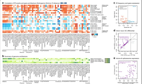
Fig. 4Relationship between gene structure and sequence composition and ES.aHeatmap representing the distance between distributions of

gene architecture values for ES-positive and ES-negative exons, measured with theDstatistic of the one-sided Kolmogorov-Smirnov two-sample

test (significant ifp< 0.01; otherwise grey).Dvalues are recorded as positive/negative (blue/red) according to two one-sided Kolmogorov-Smirnov

tests with complementary alternative hypotheses: positive/negativeD(blue/red) reflects a positive/negative relationship between ES and the

given feature.bHeatmap representing the correlation between intron length and GC content across 65 eukaryotes. Positive correlations (long,

GC-rich introns, Spearman’srho> 0 andp< 0.01) are shown inblue, negative correlations inred.cHeatmap representing genome-level gene

architectural traits, for reference: intron density (introns/gene), median exon and intron length (bp), and GC content (percentage).dDifference in

intron lengths (y-axis) between homologous sites ofS. arcticacompared toC. fragrantissimaorC. owczarzaki, ranking introns according to their

length differential withS. arctica(x-axis).Black arrowsindicate the percentage of introns that are longer inS. arcticathan in the other species

(totals between brackets).eDifference in intron lengths (y-axis) between homologous sites ofV. cartericompared toC. reinhardtiiorC. variabilis,

ranking introns according to their length differential withV. carteri(x-axis).Black arrowsindicate the percentage of introns that are longer inV.

carterithan in the other species (totals between brackets).fGC content in exons (GCex) and introns (GCin) for each species in the dataset. Note

splicing typically happens for short introns flanked by long exons [50,53]. Surprisingly, however, our analysis revealed that the influence of intron and flanking exons’length on IR is not homogeneous across eukaryotes (Fig.5a): retained introns are indeed shorter than constitutively excluded ones in chordates (vertebrates and the tunicateCiona intestinalis), S. arctica,Vitis vinifera, and unicellular algae (Micromonas pusilla,Cyanophora paradoxa,Emiliania huxleyi,B. natans, orGuillardia theta); but not in most other animals, unicel-lular holozoans, fungi, or other protists that also exhibit high IR frequencies (Additional file 1: Figure S6). The ratio of intron-to-exon length has a similarly uneven relationship with IR. Across most eukaryotes, however, introns in genes with lower intron densities (introns/ gene) were generally more prone to IR, as expected. Overall, the dominance of IR in a given genome does not seem to be determined by a straightforward rela-tionship between intron length and density. Instead, positive or negative associations can be found in a lineage- or species-specific manner.

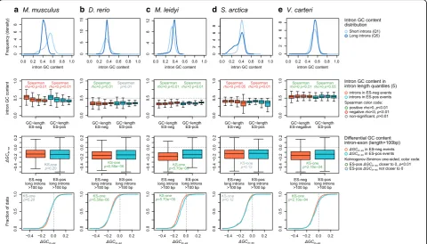
We also used the GC content of introns (GCin) and exons (GCex) and its differential (ΔGCin–ex=GCin−GCex) to examine the effect of global sequence composition in AS within each species. It has been proposed that, in species with extremely long introns (e.g., mammals and G. gallus), a differential in GC content between exons (GC-richer) and flanking introns (AT-richer) can act as a compositional mark to assist the recognition of splice sites [52]. Considering that GCin is lower than GCex in all but one eukaryote in our dataset (Fig. 4f), GC differentials in ES-positive exons could be expected to take negative values (ΔGCin-ex < < 0), particularly for long introns. However, we found that this is far from being a general rule, as we observed multiple intricate associations between ΔGCin-ex, ES frequency, and intron length that vary across eukaryotes.

First, we found that the overabundance of ES-positive exons in genic environments where ΔGCin–ex < < 0 (i.e., GC-rich exons flanked by AT-richer introns) occurs only in vertebrates and the annelidC. teleta(Fig.4a). In these

c a

b

d

e

Fig. 5Relationship between gene structure and sequence composition and ES.aHeatmap representing the distance between distributions of

gene architecture values for IR-positive and IR-negative introns, measured with theDstatistic of the one-sided Kolmogorov-Smirnov two-sample

test (significant ifp< 0.01; otherwise grey).Dvalues are recorded as positive (blue) or negative (red) according to two one-sided

Kolmogorov-Smirnov tests with complementary alternative hypotheses.bHeatmap representing genome-level gene architectural traits, for reference: intron

density (introns/gene), median exon and intron length (bp), and GC content (percentage).cVolcano plot representing the Spearman’s rank

correlation coefficient (rho,x-axis) between IR frequency and transcript expression levels (cRPKM) in IR-positive genes. Significance threshold of

p< 0.01 (y-axis, log-scale).dMean intron–exon GC differential in IR-negative (x-axis) and IR-positive (y-axis) introns. The majority of eukaryotes lie

above the diagonal (purple) as they have lower differentials in their IR-positive introns, i.e., IR occurs in GC-homogeneous introns.eCorrelation

animals, ES-positive exons were also found to be prefer-entially flanked by long introns (see above). However, long introns flanking ES-positive exons were only found to be AT-enriched in mammals andG. gallus(Spearman rho < 0 and p < 0.01; Figs. 4b and 6a, b). Second, a number of other eukaryotes (e.g., S. ciliatum,S. arctica, orO. sativa) exhibited a similar correlation between long and AT-rich introns genome-wide (red in Fig.4b), but not the concomitant association between strong GC differen-tials (ΔGCin–ex < < 0) and ES (Figs. 4a and 6e). Third, ES-positive exons in nearly all non-vertebrate eukaryotes were surprisingly biased towards regions where introns and exons have similar GC content (i.e., ΔGCin–ex~ 0; Fig.6b–e). This latter pattern was highly unexpected, as it matches that described for IR events in human [52], which we also observed for IR for most (yet not all) eukaryotes in our dataset (Fig.5a, d). Altogether, these results reveal complex lineage-specific interplays among GC content, intron length, and ES frequency, which cannot be generalized among eukaryotes (Fig.6).

We have also examined the effect of whole-transcript expression levels on AS. In the majority of eukaryotes, IR-positive introns are preferentially found in lowly expressed transcripts (Fig. 5a). This result is predicted by two alternative and non-mutually exclusive hypoth-eses. On the one hand, IR has been widely associated

with down-regulation of gene expression via NMD [16]. On the other hand, random splicing errors are more prone to affect lowly expressed genes, given its reduced fitness cost [49]. A closer inspection of IR-positive introns alone also recovered a widespread correlation between high IR rates (rIR,in) and lower expression levels in 28 out 37 species where the relationship was signifi-cant (Fig. 5c, Additional file 1: Figure S20;p< 0.01 and rho < 0 in Spearman’s rank correlation test). This result had been previously described in mammalian transcrip-tomes [16] and can thus be extended to all eukaryotes.

Finally, we investigated the relationship between the relative expression of core spliceosomal components and IR and ES frequency genome-wide. Since efficient splicing depends, in principle, on the sufficient expression of spliceosomal components [58, 59], we asked whether low relative expression of core factors correlated with higher ES and/or IR frequencies at the species level (Additional file 1: Figure S21A–C). Using a rank-based score to measure relative spliceosome expression (see “Methods”), we identified a negative association between spliceosome expression and IR frequency (Additional file1: Figure S21B). This result suggests that species-wide IR levels, which do not follow a phylogenetic pattern (Additional file1: Figure S6), could be at least partly ex-plained by the competition among unspliced transcripts

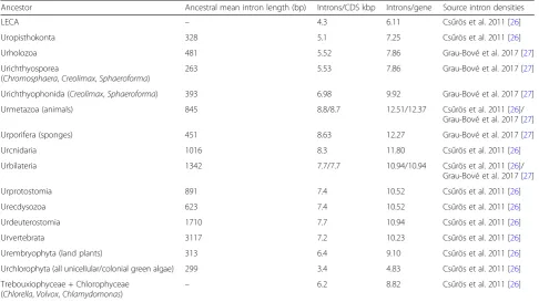
Table 1Intron mean lengths and densities in ancestral eukaryotic genomes

Ancestor Ancestral mean intron length (bp) Introns/CDS kbp Introns/gene Source intron densities

LECA – 4.3 6.11 Csűrös et al. 2011 [26]

Uropisthokonta 328 5.1 7.25 Csűrös et al. 2011 [26]

Urholozoa 481 5.52 7.86 Grau-Bové et al. 2017 [27]

Urichthyosporea

(Chromosphaera,Creolimax,Sphaeroforma)

263 5.53 7.86 Grau-Bové et al. 2017 [27]

Urichthyophonida (Creolimax,Sphaeroforma) 393 6.98 9.92 Grau-Bové et al. 2017 [27]

Urmetazoa (animals) 845 8.8/8.7 12.51/12.37 Csűrös et al. 2011 [26]/

Grau-Bové et al. 2017 [27]

Urporifera (sponges) 451 8.63 12.27 Grau-Bové et al. 2017 [27]

Urcnidaria 1016 8.3 11.80 Csűrös et al. 2011 [26]

Urbilateria 1342 7.7/7.7 10.94/10.94 Csűrös et al. 2011 [26]/

Grau-Bové et al. 2017 [27]

Urprotostomia 891 7.4 10.52 Csűrös et al. 2011 [26]

Urecdysozoa 623 7.4 10.52 Csűrös et al. 2011 [26]

Urdeuterostomia 1710 7.7 10.94 Csűrös et al. 2011 [26]

Urvertebrata 3117 7.2 10.23 Csűrös et al. 2011 [26]

Urembryophyta (land plants) 313 6.4 9.10 Csűrös et al. 2011 [26]

Urchlorophyta (all unicellular/colonial green algae) 299 3.4 4.83 Csűrös et al. 2011 [26]

Trebouxiophyceae + Chlorophyceae (Chlorella,Volvox,Chlamydomonas)

– 6.2 8.82 Csűrös et al. 2011 [26]

Mean intron lengths estimated from phylogenetically independent comparisons of descendant species (see“Methods”; Additional file1: Figure S24). Intron

densities (taken from [26,27]) are reported as introns/CDS kbp and introns/gene (by multiplying by the average CDS length [1422 kbp] of all organisms in our

for access to the available spliceosomal machinery [58,59] in a species- and/or sample-dependent manner. On the other hand, we found a mild, unexpectedly positive association of core spliceosomal expression with ES frequency (Additional file 1: Figure S21C). However, this result is likely due to the strong correlation found between relative spliceosomal expression and the total number of introns (Spearman’srho= 0.612,p= 1.28e−7; Fig. 5e) and intron density (Additional file 1: Figure S21D), which were also positively correlated with ES frequencies (Fig. 4). Thus, relative expression of core spliceosomal components seems adjusted to the number of introns to be spliced in each species.

In summary, ES events across eukaryotes were globally associated with short exons flanked by longer introns, and with weak 5′and 3′splice sites. Inasmuch as these features are more common in animals and plants than in most eukaryotes, we can expect higher ES frequencies in these multicellular lineages.

Dating ES transitions in ancestral Holozoa genomes

The relationships between ES and genomic features de-scribed above were highly consistent among Holozoa

(animals and their closest unicellular relatives), which suggests that these architectural and sequence effects in-fluenced ES frequencies not only in extant organisms but in their extinct ancestors as well. We thus reasoned that these relationships could be used to predict the inci-dence of ES in ancestral genomes, provided that their genome architectures could be approximated.

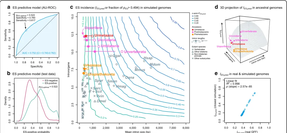
For this purpose, we first trained a binomial logistic regression model (see “Methods”) that classifies arbi-trary exons as either ES-positive or -negative accord-ing to their overall gene architecture, assignaccord-ing them an ES-positive probability (pES). We used data from a selection of 24 eukaryotes with multiple animals and holozoans (Additional file1: Figures S22 and S23) and ascertained their sensitivity and specificity by calculat-ing the ROC curve of the classifier (Fig. 7a) and the area underneath (AU-ROC = 0.752, 95% CI = 0.743–0.762). This AU-ROC value indicates a clearly better-than-random classifier and compares with similar AS predictors previ-ously developed for more taxonomically restricted contexts, such as IR in mammals (AU-ROC = 0.79) [16] and ES in vertebrates (AU-ROC = 0.79–0.87 in individual species) [51]. In addition, it shows that gene architecture is a

a b c d e

Fig. 6Representative patterns of the inter-relationships between GC content and AS. For selected eukaryotes (a–e), we plotted the distribution of

GC content (percentage) in long and short introns (first row); the distribution of GC content in introns sorted according to their length (five

quantiles, Q1–5), and ES status (negative and positive;second row); and the differential between intron and exon GC content in long introns (Q5)

of ES-positive and ES-negative events, using box plots (third row) and empirical cumulative distribution functions (fourth row). In thesecond row,

we used Spearman’s rank correlation coefficient to test the association between intron length and GC content (significant atp< 0.01). In thethird

andfourth rows, we used Kolmogorov-Smirnov one-sided test to test whether ES-positive introns had higherΔGCin–exthan ES-negative ones

consistent predictor of ES events. The highest combined sensitivity and specificity were attained when the ES-positive probability threshold (pES) was set at 0.522 (Fig.7b).

Next, we used this classifier to compare ES levels from an-cestral genomes, using a topographic map of the predicted ES incidence based on genomic architectural traits (Fig.7) from 1600 genomes simulated by combining initial assump-tions of mean intron density (range 0.5–15 introns/gene) and mean intron length (range 10–8000 bp). For each simu-lation, we generated 10,000 internal exons with their corre-sponding gene architectures (see“Methods”for details) that were analyzed with the classifier to assign them an ES-positive probability (pES). Then, we approximated the in-cidence of ES in each simulated genome by calculating the fraction of exons with pES over the optimal threshold (pES > 0.522; henceforth IES). An examination of ES incidences across the spectrum of simulated ancestral genomes revealed that genomes with higher intron densities and lengths have higherIESvalues (Fig.7c, d), as expected from transcriptomic analyses of extant species (Fig. 4a, b). To assess the accuracy of our simulated genomes, we

compared their IES values with those obtained from the most similar real genome in our dataset (in terms of intron density and mean length), finding a linear correlation (linear fitR2= 0.996, slopep= 1.25e−76; Fig.7e).

Then, we used this predictive framework to analyze ES transitions in animals by comparing the incidence of ES in reconstructed premetazoan and postmetazoan ancestors (Fig.7c). To do so, we used previously pub-lished estimates of intron density in ancestral genomes obtained by comparative genomic analyses [26, 27], which reported an increase in intron density from 7.85 to 12.37 introns/gene between the origin of Holozoa (Urholozoa) and animals (Urmetazoa) (Table 1). As a proxy for ancestral intron lengths, we used means obtained from extant species’ phylogenetically inde-pendent contrasts [60] (see “Methods”; Additional file 1: Figure S24). Under these assumptions, the Urmetazoa (12.37 introns/gene of ~ 850 bp mean length) would have anIES ~ 0.30 (Fig.7c). Conversely, the intron-poorer Urholozoa would reach IES ~ 0.30 only if it had an average intron of > 1000 bp, which exceeds by an order of magnitude the average intron

e d c

a

b

Fig. 7Prediction of ES incidences in ancestral genomes.aReceiver operating characteristic (ROC) curve of a binomial logistic regression model of ES prediction derived from 11 gene architectural features, 22 species, and a dataset of 18,678 exon skipping events for training and testing (see“Methods”). AU-ROC value (0.752) is reported with 95% confidence interval. The non-pale blue dotmarks the optimal probability threshold

(0.522) corresponding to the maximum sum of sensitivity (0.617) and specificity (0.760).bES-positive probability distributions of the test dataset,

containing 9318 exons with known ES status (50% positive, ingreen; 50% negative, inmaroon). Thedotted linemarks the optimal probability

threshold (0.522; see above).cContour plot representing ES incidences (IES,zaxis) across 1600 simulated genomes of varying mean intron sizes

(horizontal) and intron densities (vertical).IESis defined as the fraction of exons in a given simulation withpES> 0.522.Grey marksrepresent extant

species positions in the intron size and density dimensions.Red/pink/orange-colored dotsrepresent estimates of ancestral premetazoan and

metazoan genomes. Ancestral intron densities from [26,27] (Table1); ancestral intron length distributions are represented by the mean, median,

and first and third quartiles (Table1, Additional file1: Figure S24; see“Methods”).d3D projection ofc, withIES, (z-axis), intron sizes (x-axis), and

intron densities (y-axis). Eachdotrepresents an estimation of a genome (intron density and mean intron length).eCorrelation between theIES

values obtained from analyzing real genome architectures with the predictive classifier (x-axis) and its closest equivalent from the spectrum of

lengths of extant unicellular holozoans (120–571 bp; Additional file 1: Figure S2) [27] and our ancestral estimation (~ 481 bp). Therefore, under reasonable assumptions for ancestral genome architecture, the unicellular ancestors of animals likely had lower ES levels than the Urmetazoa (Fig.7c, d).

This same line of reasoning can be applied within animals. Since the Urmetazoa (12.36 introns/gene, ~ 850 bp), intron loss processes occurred in the ancestral cnidarians, porifer-ans, bilateriporifer-ans, and vertebrates (Table1) [26,27]. Therefore, to sustain an increase in ES levels relative to the Urme-tazoan, these lineages should have undergone intron length-ening processes. This was probably the case already in early bilaterians (IES~ 0.40 if mean intron length ~ 1300 bp) and, with higher certainty, in vertebrates (IES ~ 0.60 if mean intron length ~ 3100 bp; Fig.7c, d). On the other hand, our results do not support bilaterian-like ES enrichments in the early branching animal ancestors Urcnidaria and Urporifera: although they had high intron densities, they likely had shorter introns compared to the Urbilaterian (Table1), thus yielding lowerIESvalues (Fig.7c, d).

Therefore, we hypothesize that the moderately high ES in certain non-bilaterian eukaryotes appear concomitantly with recent, species-specific changes in their gene archi-tecture. One possible example isH. magnipapillata, which has undergone a recent, intra-genus genome size expan-sion [61,62] that could help explain its enlarged introns (Fig. 1b). Similarly, ichthyosporeans attained high intron densities independently of animals [27] (Table1), and the longer introns found in species like S. arctica appear to have been recently acquired too (Fig.4d). Altogether, pre-diction of ES incidences from ancestral reconstructions and comparison with extant species are consistent with the increase in ES frequency observed in metazoans, particularly from bilaterian ancestors.

Discussion

We performed a comparative survey of AS frequencies in 65 eukaryotes to understand the evolutionary dynam-ics of this layer of gene regulation. Our analysis revealed that ES and IR events can be found, at varying frequen-cies, in transcriptomes from all major eukaryotic groups (Opisthokonta, Amoebozoa, Virdiplantae and Crypto-phyta, SAR and HaptoCrypto-phyta, and Excavata). This result thus provides further support for an early emergence of dual AS—i.e., involving both ES and IR—in eukaryotes [18,33,34]. Given the generally higher prevalence of IR in all eukaryotic super-groups (Fig.2a, b, Additional file1: Figure S6), LECA likely exhibited an IR-dominated AS profile as well.

Since its early origin in LECA, the incidence of ES has varied between different eukaryotic groups. Our analysis of ES frequencies across multiple species revealed higher ES frequencies in multicellular animals (particularly

vertebrates and other bilaterians) and, to a lesser extent, plants. While most other eukaryotes maintain lower ES levels, a number of punctual exceptions have surfaced—e.g., the ichthyosporean S. arctica or the colonial chlorophyte V. carteri [38] (Fig. 2). Con-versely, other major lineages like fungi or amoebozo-ans exhibit comparatively low ES levels.

In most ES-rich eukaryotes, we identified a set of gene architectural features that influence the frequency of AS at the gene level: the heterogeneity of 5′ and 3′ splice sites, the length of exons and their flanking introns, and its correlate regarding intron density. These architectural traits were globally coherent across eukaryotic lineages, especially in animals and plants (Fig. 4a). In particular, the mode of splicing by ‘exon definition’, which posits that short exons flanked by long introns are enriched in ES events [50, 53], is relevant in most eukaryotic transcriptomes with sufficient ES levels analyzed here, except for E. siliculosusand B. natans. These properties are more common in intron-rich organisms with hetero-geneous splice sites [18,34]. Overall, this result suggests a non-deterministic ‘soft code’ that influences ES rates across eukaryotic lineages.

Furthermore, if the effect of gene architecture on ES is widespread and coherent across eukaryotes, we can infer that it was also relevant in their ancestors. Thus, we took advantage of the pan-eukaryotic ‘soft code’ of ES determination to investigate the timing of ES transitions in animals and their unicellular ancestry. Specifically, we quantified the relationship between gene architecture and ES on extant eukaryotes and projected these effects into the past with a predictive framework (Fig. 7c, d). We propose an early ES enrichment in the Urmetazoa concomitant with the origin of multicellularity, followed by further enrichment in bilaterians and vertebrates. The ES transition in early animals would come as a conse-quence of changes in genome architecture, as large ge-nomes with high intron densities and long intronic segments became more common in animals [26, 27, 69] than in their unicellular holozoan relatives [27,57,70–72]. Remarkably, most animals showed high fractions of 3n exons among their ES events, but this was not observed in plants or other eukaryotes (Fig.3b, c). Thus, the pres-sure to maintain ORFs in the event of ES seems an animal-specific trait. Interestingly, even animals with lower ES frequencies (such as non-bilaterians) or that have secondarily simplified intron–exon architectures (e.g.,C. elegans andD. melanogaster) often have strong 3n biases in their ES profiles. Thus, it is conceivable that a protein isoform-enabling 3n bias already existed in the Urmetazoa, before the major increase in ES frequency occurred in bilaterians (Figs. 2 and 7). If so, these increases were likely more easily recruited to function-ally diversify their proteomes, perhaps contributing to the selection of more ES-prone genome architectures, establishing a positive feedback loop. Moreover, it is possible that other regulatory features that are charac-teristic of bilaterians, such as the high prevalence of long-range enhancer–promoter interactions [73], may have also contributed to longer intron sequences and thus to more ES-prone genome architectures.

On the other hand, neither unicellular holozoans (Fig. 2) nor the unicellular ancestors of animals (Fig. 7) seem to have had ES-rich transcriptomes with 3n exon biases. Therefore, AS-mediated isoform production was a largely irrelevant phenomenon during the unicellular ancestry of animals (since the Urholozoa to the origin of multicellularity), an evolutionary period that was other-wise fecund in other sources of gene innovation [27].

Conclusions

We find that the influence of gene architectural traits in the frequencies of IR and ES is globally conserved across all eukaryotic lineages. Thus, gene architecture (i.e. the lengths of introns and exons, splice site definition, intron density, etc.) is the basis of a ‘soft’ pan-eukaryotic cis-regulatory code for AS determination that affects

both extant and ancestral genomes. This result em-phasizes the effect of long-term genome evolutionary patterns in shaping AS, a fast-changing transcriptome regulatory layer. In that regard, we identify multiple ES transitions coinciding with the evolution of ES-favourable genome architectures – e.g. in animals and plants, but also in more restricted taxonomic contexts such as the ichthyosporean S. arctica.

Our taxon-rich analysis confirms that animal tran-scriptomes have a unique AS profile. Quantitatively, ex-tant animals exhibit the highest ES frequencies among eukaryotes as a consequence of cumulative ES enrich-ments in the Urmetazoa and, above all, the Urbilateria. Furthermore, from a qualitative perspective, the earliest animals became enriched in frame-preserving ES events, which is essential for widespread isoform-mediated proteome diversification. Thus, our observations suggest that the unparalleled increase in ES frequencies of mod-ern bilaterians (including vertebrates) is a consequence of the interplay between the complexification of animal genome architectures, on one hand, and the co-option of ES events for regulated proteome expansion, on the other.

Methods

Sources of genome and transcriptome data

We assembled a dataset consisting of genome assemblies and annotations from 65 eukaryotic species for which high-coverage Illumina RNA-seq data were already available or for which we generated de novo data (Additional file 1: Figure S1 and below). We retrieved the genomic coordinates of genes, transcripts, and exon sequences for each genome from associated GFF annotation files. If more than one isoform per gene was annotated, the longest CDS was considered to be the canonical transcript (a proxy with ~ 90% corres-pondence with proteomics-driven main isoform selec-tion [74]). In order to homogenize the experimental procedures used to build each RNA-seq library, we used (i) poly(A)-selected libraries only, (ii) either single-end or the forward reads of paired-end data, and (iii) trimmed reads to a length of 50 bp if they were longer (using FASTX Toolkit [75]). In species where RNA-seq experiments included more than one sample (replicates, time series, growth conditions, etc.), all reads were pooled into a single FASTQ file.

organisms (T. adhaerens, artificial sea water at 25 °C). RNA was extracted using Trizol reagent (Life Technolo-gies, Carlsbad, CA, USA) with a further step of Dnase I (Roche) to avoid contamination by genomic DNA, then purified using RNeasy columns (Qiagen). We sequenced paired-end libraries of 50 (N. gruberi, 276,095,412 reads;S. arctica, 218,701,756 reads) or 125 bp (T. adhaerens, 84,583,746 reads) with an insert size of 250 bp. Libraries were constructed using the Trueseq Sequencing Kit v4 (Illumina, San Diego, CA, USA). The libraries were se-quenced in one lane of Illumina HiSeq 2000 (N. gruberi, T. adhaerens) or 2500 (S. arctica) at the CRG genomics fa-cility (Barcelona).

Detection and quantification of exon skipping and intron retention events

We adapted and expanded the computational framework previously developed [36, 51] to detect and quantify ES and IR (graphical summary in Additional file1: Figure S3), as follows.

Exon skipping detection

For each group of three consecutive exons in the genome (exon triplet), we built a composite of exonic junctions consisting of (i) 42 bp from the 5′end of the first exon and 42 bp from the 3′ end of the second exon (E1–E2 junction); (ii) 42-bp fragments from the 5′end of the first exon and the 3′ end of the third exon (E1–E3); and (iii) 42-bp fragments from the 5′end of the second exon and the 3′end of the third exon (E2–E3). Hence, each triplet consisted of two inclusion junctions (E1–E2 and E2–E3) and one that skipped the middle exon (E1–E3). If any exon was shorter than 42 bp, the entire length of the exon was used, and the resulting junction sequence would be shorter than 84 bp.

Then, we computed the effective mappability of each junction in order to exclude exon–exon boundaries where RNA-seq mapping would be unreliable [76]. Spe-cifically, we (i) built an artificial RNA-seq library consist-ing of all the possible reads derived from each junction in a 50-bp sliding window; (ii) mapped these reads to the original junctions using bowtie v1.1.2, allowing a maximum of two mismatches (−v 2) and no multiple alignments (−m 1) [77]; and (iii) removed all junction triplets for which at least one triplet had < 20 effectively mappable positions (maximum is 35 for 50 bp reads, and≥8 positions mapped from each exon). Then, we aligned the pooled RNA-seq libraries to the remaining exon triplets with bowtie and the same parameters as above. We corrected the number of mapped reads by dividing the read counts by the ratio obtained from div-iding the mappable positions of that junction (20–35 bp) and the maximum theoretical mappability (35 bp).

The ES rate of each middle exon (rES) was then com-puted as follows:

rES¼

mE1E3

mE1E2þmE2E3

ð Þ=2þmE1E3

where m denotes the mappability-corrected number of reads mapping in the E1–E2, E2–E3, and E1–E3 junc-tions. We classified exon junctions into three categories: (i) ES-positive if mE1E2+mE2E3 +mE1E3 > 10,mE1E2> 2,

mE2E3 > 2, mE1E3 > 1, and rES ≥10% but < 90%; (ii) ES-negative if mE1E2 + mE2E3 + mE1E3 > 10, mE1E2 > 2,

mE2E3 > 2, mE1E3 ≥0 but rES< 10%; and (iii) non-classifiable if any condition was not fulfilled.

Intron retention detection

For each intron of the genome, we built three junction sequences consisting of (i) 42 bp from the 5′end of the first exon and 42 bp from the 3′end of adjoining intron (E–I junction); (ii) 42-bp fragments from the 5′ end of the first exon and the 3′end of the second exon (E–E); and (iii) 42 bp fragments from the 5′end of the intron and the 3′ end of the second exon (I–E). Hence, each intron triplet had one spliced junction (E–E) and two retention junctions that spanned the intron ends (E–I and I–E), all of them 84 bp long (or less, if any exon or intron was shorter than 42 bp).

The mappability of each exon–intron junction was computed as specified above for ES junctions, also discarding cases with < 20 effectively mappable positions. We then aligned the same pooled RNA-seq data to the remaining exon–intron junctions using bowtie, and cor-rected the number of mapped reads.

The IR rate of each intron (rIR) was computed as follows:

rIR¼

mIEþmEI

ð Þ=2

mEEþðmIEþmEIÞ=2

where m denotes the mappability-corrected number of reads mapping in the I–E, E–I, and E–E junctions. Finally, we classified intron junctions in three categories: (i) IR-positive ifmIE+mEI+mEE > 10,mIE> 1,mEI> 1,

mEE > 2, and rIR ≥ 10% but < 90%; (ii) IR-negative if

mIE + mEI + mEE > 10, mIE ≥0, mEI ≥0, mEE > 2, and

rIR.in< 10%; and (iii) non-classifiable if any condition was not fulfilled.

ES and IR detection pipeline quality control

(paralogy, exon/intron lengths, repetitive genomes) could affect RNA-seq mapping in certain species and thus bias downstream analyses.

We analyzed the fraction of junctions with > 20 effective mappable positions (mappability filter, Additional file 1: Figure S25A, B), finding no evidence of taxonomic biases in any particular eukaryotic group. A few phylogenetically unrelated species exhibited low survival rates (e.g., Selaginella moellendorffi and E. huxleyi). This general mappability filter was then decomposed in its different components. First, we assessed the fraction of exons and introns from each genome that had the minimal required length to survive the mappability filter (i.e.,≥27 bp), find-ing no bias in any species (Additional file1: Figure S25C, D). Next, we examined which mapping filters (i.e.,bowtie multiple mapping [−m 1] or excess of mismatches [−v 2]) caused ES or IR junction removal in each species (Additional file1: Figure S25E, F), finding that peaks in S. moellendorffi and E. huxleyi were mostly due to multiple mapping. Multiple mapping is likely caused by abundant recent gene duplications in these two species. Indeed, both S. moellendorffi and E. huxleyihad a high fraction of intron-bearing genes with recent paralogous sequences (> 99% or > 95% amino acid sequence identity, and > 90% reciprocal alignment coverage, calculated with diamond [78]; Additional file 1: Figure S25G, H). Finally, we found that some species also had a rela-tively high number of uncalled bases (N) in their exon–exon or intron–exon junctions (most notably O. sativa but also S. moellendorffi; Additional file 1: Figure S25I, J), which can partly explain the lower survival rates in these species after the mappability filter (Additional file1: Figure S25A, B).

Overall, these quality control analyses show that the compounded effect of genome architectural traits (recent duplication, uncalled bases, and repetitive se-quences hindering RNA-seq mapping) only affected individual species and did not systematically affect ES or IR detection in any large group of eukaryotes.

Transcriptome-wide quantification of AS levels

In order to measure the average frequency of ES at the species level, we divided each species’ set of classifiable exon triplets into 100 bins of 100 triplets, and calculated the per-triplet frequency of ES from 10,000 randomly chosen reads for each bin (selected among those mapping to the in bin’s exon–exon junctions, or a mean sequencing depth of ~ 20×). The average ES rate of each bin i(rES,i) was recorded to obtain a species-level distribution of ES frequencies (FES,sp). An analogous measurement was used to calculate the distribution of species-level IR frequencies (FIR,sp) from 100 bins, 100 triplets, and 10,000 reads per bin (mean sequencing depth ~ 20×). This process is summarized in Additional file1: Figure S3C. It should be

noted that comparisons amongFIR,spare more susceptible to technical variability derived from library preparation than those amongFES,sp, since differences in the efficiency in poly(A)+ selection are only expected to significantly affectFIR,spestimates.

Statistical comparisons of poolings of species-level FES,sp distributions (Fig. 2c–f) were done using one-sided Kolmogorov-Smirnov tests. Differences between intra-species replicates (Additional file 1: Figure S7) were assessed with Wilcoxon rank-sum tests. All statistical contrasts were done with Rstats[79].

ES frequency analysis was re-assessed by using (i) down-sampled RNA-seq experiments (to 2×, 5×, 10×, and 15× sequencing depths, by random read selection; Additional file 1: Figure S10); and (ii) individual tissue-level samples from selected animal (H. sapiens, 2× M. musculus, M. domestica,O. anatinus,G. gallus,X. tropicalis,D. rerio,S. ciliatum) and plant species (A. thalianaand M. polymor-pha) (Additional file1: Figure S13A). Original sequencing depths in the ES and IR triplets junctions are available in Additional file1: Figure S25K, L.

Analysis of gene features: architecture, splice sites and expression levels

For each exon or intron analyzed, we recorded sequence and architectural parameters at the gene and AS event levels. At the gene level, we studied the following parame-ters: gene length, CDS length (all exons), total number of introns in the gene (intron density), position of the exon/ intron within the gene sequence (base pairs from starting codon), and total length of all introns with respect to exons (ratio). At the AS event level, we recorded the length of the individual exon and flanking introns (for ES) or intron and flanking exons (for IR), and the ratio be-tween them (intron/exon lengths); the GC content of exons and flanking introns (for ES) or introns and flanking exons (for IR), and the differential between them (ΔGCin–ex=GCin–GCex), and a boolean variable describ-ing whether the length of the alternative exon/intron was divisible by three (1 = true, 0 = false). These features were derived from the GFF annotation and genome sequence (data sources in Additional file1: Figure S1).

In addition, we analyzed the conservation degree of 5′ and 3′ splice sites when compared to species-specific consensus. For each species, we built position-weighted matrices (PWM) from the alignments of all 3′(23 bp, 20 from the intron and 3 from the exon) and 5′ (9 bp, 3 from the exon and 6 from the intron) splice sites using the consensus matrix function in theBiostringsR library [80]. Then, for each individual splice site in the genome, the distance from the PWM consensus was calculated. Splice sites were delimited as in [81].

aligning the pooled RNA-seq data for each species to the genome-predicted transcript sets using bowtie (longest transcript per gene only, see above) and calculating transcript-specific effective mappabilities as detailed above [76].

Statistical analysis of AS frequency and gene features

For each species and for each of the quantitative se-quence and architectural features listed above, signifi-cant differences between the values taken by the IR-/ ES-positive triplets and the IR-/ES-negative triplets were evaluated using two independent one-sided Kolmogorov-Smirnov two-sample tests with comple-mentary alternative hypotheses: first, we tested whether the empirical cumulative distribution of the IR-/ES-po-sitive events lied above the IR-/ES-negative events’ values (signaling a positive relationship between IR/ES and the given feature); second, we tested whether it lied below (i.e., for a negative relationship). We used the Kolmogorov-Smirnov distance (D statistic) to measure the distance between distributions. D was recorded as positive ifp< 0.01 in the first test, negative ifp< 0.01 in the second one, or as NA if it was not significant in any test or contradictorily significant. The resulting matrix was plotted using the heatmap.2 function in the R gplotsv3.0.1 library [82].

To further investigate the relationship between gene expresion levels and IR, we also tested the significance of monotonic correlations between cRPKMs and AS rates using Spearman’s rank correlation coefficient (rho, significant for p< 0.01).

Finally, we tested if the frequency of 3n divisible lengths in IR-/ES-positive events significantly differed from that of IR-/ES-negative (i.e., constitutive) events using Fisher’s exact test (significant forp< 0.01, except if otherwise stated). All statistical analyses were done with Rstatslibrary [79].

The relationships between gene architectural traits and ES and IR events were re-assessed by using (i) down-sampled RNA-seq experiments (to 2×, 5×, 10× and 15× sequencing depths, by random read selection; Additional file1: Figures S17 and S18); and (ii) individual tissue-level samples from selected animal (H. sapiens, M. musculus, M. domestica, O. anatinus, G. gallus, X. tropicalis, D. rerio, S. ciliatum) and plant species (A. thaliana and M. polymorpha) (Additional file1: Figure S13B, C). Original sequencing depths in the ES and IR triplets junctions are available in Additional file1: Figure S25K, L.

Prediction of ES incidence using gene architectural features

Using our binary classification of positive/negative ES events, we created a binomial logistic regression model

for a selection of representative eukaryotes with high ES frequencies. First, we selected 18,678 events with known gene architecture (devised to include an equal number of positive and negative events) from 24 representative eukaryotic species (Additional file 1: Figure S22). We used (i) 12,452 positive and negative ES events (two-thirds of the dataset) as the binary-dependent vari-able, and (ii) 11 quantitative gene traits and a Boolean factor indicating 3n divisibility as independent predictors (Additional file 1: Figure S22). The binomial logistic re-gression was built using the generalized linear model function from R stats library [79]. The predictive per-formance of each model was estimated with the area under its corresponding ROC curve (AU-ROC), calcu-lated using an independent test subset (6226 events, one-third of the dataset) with the pROC R library [83]. An optimal probability threshold was selected by maximizing the sum of specificity and sensitivity (pES,optimal = 0.522). We assessed the significance of the model’s coefficients with the Z-statistic signifi-cance according to the Wald test and its correspond-ing ANOVA deviance table with sequential Chi-square tests (Additional file1: Figure S22).

The predictive model of ES was applied to a set of 1600 simulated genomes with varying intron densities (0.5–15 introns/gene range, 40 regular intervals) and mean intron sizes (10–8000 bp range, 40 intervals at cubic distances). Each simulated genome contained 20,000 genes of which at least 10,000 were multi-exonic (depending on its input intron density).

For each simulated genome, gene architectures were drawn from the empirical distributions derived from 10,000 randomly selected genes from each of the 30 repre-sentative eukaryotes. Specifically, we used log-normal dis-tributions for the lengths of CDS (mean = 1422 bp), 5′ and 3′ introns (mean = input mean intron length), genes (mean = CDS length + input mean intron length × input mean intron density), and exons (mean = CDS length/ number of introns per gene); and normal distributions of 5′ splice site (mean = empirical) and 3′ splice site (mean = empirical) scores. For all normal or log-nor-mal distributions, the standard deviations were obtained from the empirical distributions. See Additional file 1: Figure S23 for a complete report of means and standard deviations for each distribution and a list of species employed. All variables were esti-mated using maximum-likelihood fitting of univariate distributions as implemented in the fitdistr utility of the R MASS library [84], and each set of simulated gene architectures was built using the normal or log-normal distributions implemented in R stats [79].

binomial logistic regression model to obtain exon-wise ES-positive probabilities (pES). In simulated genomes with low intron densities, the number of internal exons (i.e., with two flanking introns) was sometimes less than 10,000 (for the lower bound of 0.5 introns/gene, 7864 internal exons were retrieved on average).

To estimate the incidence of ES across the spectrum of simulated genomes, we calculated the fraction of exons in each simulation with pES > 0.522 (the optimal probability threshold according to the ROC curve with real test data), orIES. The relationship betweenIES, mean intron size, and intron density was investigated using a contour map and its corresponding 3D projection, pro-duced with the Rgraphics[79] andakima libraries [86], respectively.

Then, we overlaid the resulting contour map with esti-mations of ancestral genomes’intron density and length distributions. Ancestral intron densities were obtained from [26,27] (Table1). Ancestral intron length distribu-tions were estimated using phylogenetically independent contrasts (PIC) [60, 87] as implemented in the R ape library [88]. Specifically, we calculated mean, median, and first and third quartiles of the ancestral intron length distributions, using PIC analysis of the descend-ant nodes (e.g., Urcnidaria median value corresponds to the phylogeny-controlled medians of the three extant cnidarians in our dataset; available as Additional file 1: Figure S24). In order to account for the phylogenetic relationships as required in PIC analysis [60, 87], we built a phylogenetic tree of the 65 eukaryotes in our dataset with 429 single-copy pan-eukaryotic orthologs from the BUSCO database [89] with IQ-TREE v1.5.1 [90]. For each of the 429 BUSCO orthologs and 65 organisms, we searched the best-matching protein in each predicted proteome with hmmsearch [91], which were aligned with MAFFT v7.245 (L-INS-i algorithm with up to 1000 refinement iterations) [92] and trimmed with the trimAL automated algorithm [93]. Then, we concatenated all 429 trimmed alignments in a multi-gene alignment (149,809 amino acid positions) that was analyzed with IQ-TREE using the LG + G4 model and a constrained phylogenetic tree as a reference (manually built from previous phylogenomic analyses [27, 94–97]; see Additional file1: Figure S24).

Length distribution of homologous introns in holozoans and chlorophytes

To test whether S. arctica and V. carteri have length-ened or shortlength-ened their introns, we compared the length distributions of one-to-one homologous introns between them and their close relatives. First, we built two databases of orthologous genes: for unicellular holozoans (using predicted proteins of S. arctica and C. fragrantissimaplus C. owczarzakias outgroup) and

chlorophytes (using V. carteri and C. reinhardtii, plus Chlorella variabilis as outgroup), using in both cases Orthofinder v2.1.2 [98] with MCL inflation = 2.1 [99]. Please note that, although C. perkinsii (ichthyospor-ean) is a closer outgroup for the holozoan analysis than C. owczarzaki (filasterean), the former species’ intron contents are heavily reduced, whereas the latter shows a remarkable level of intron site conservation despite the high phylogenetic distance with ichthyos-poreans [27].

For each database of orthologous genes, we retrieved the transcript sequences of all single-copy orthologs present in the three species, onto which we mapped the in-transcript coordinates of all annotated introns and their length (bp). For each three-gene group, we re-trieved 40-bp-long transcript segments around each intron site (20 bp upstream + 20 bp downstream) using Bedtools v2.24.0 [100], and aligned them locally with blastn [101] to identify introns inserted in homologous transcript regions (using-task blastn-short). We consid-ered as homologous introns those alignments that fulfilled these conditions: (i) alignment length > 8 bp; and (ii) alignment spanned at least 4 ungapped bp up/ downstream the intron insertion (20th position). Then, we analyzed the intron length distribution of homolo-gous introns in pairwise species comparisons.

Conservation and expression of the core spliceosomal components