Feature selection and dimension reduction for single cell RNA Seq based on a multinomial model

M E T H O D

Open Access

Feature selection and dimension

reduction for single-cell RNA-Seq based on a

multinomial model

F. William Townes

, Stephanie C. Hicks

, Martin J. Aryee

and Rafael A. Irizarry

Abstract

Single-cell RNA-Seq (scRNA-Seq) profiles gene expression of individual cells. Recent scRNA-Seq datasets have incorporated unique molecular identifiers (UMIs). Using negative controls, we show UMI counts follow multinomial sampling with no zero inflation. Current normalization procedures such as log of counts per million and feature selection by highly variable genes produce false variability in dimension reduction. We propose simple multinomial methods, including generalized principal component analysis (GLM-PCA) for non-normal distributions, and feature selection using deviance. These methods outperform the current practice in a downstream clustering assessment using ground truth datasets.

Keywords: Gene expression, Single cell, RNA-Seq, Dimension reduction, Variable genes, Principal component analysis, GLM-PCA

Background

Single-cell RNA-Seq (scRNA-Seq) is a powerful tool for profiling gene expression patterns in individual cells, facil-itating a variety of analyses such as identification of novel cell types [1,2]. In a typical protocol, single cells are iso-lated in liquid droplets, and messenger RNA (mRNA) is captured from each cell, converted to cDNA by reverse transcriptase (RT), then amplified using polymerase chain reaction (PCR) [3–5]. Finally, fragments are sequenced, and expression of a gene in a cell is quantified by the number of sequencing reads that mapped to that gene [6]. A crucial difference between scRNA-Seq and tradi-tional bulk RNA-Seq is the low quantity of mRNA isolated from individual cells, which requires a larger number of PCR cycles to produce enough material for sequencing (bulk RNA-Seq comingles thousands of cells per sam-ple). For example, the popular 10x Genomics protocol uses 14 cycles [5]. Thus, many of the reads counted in scRNA-Seq are duplicates of a single mRNA molecule in the original cell [7]. Full-length protocols such as SMART-Seq2 [8] analyze these read countsdirectly, and several

*Correspondence:rafa@ds.dfci.harvard.edu

1_{Department of Biostatistics, Harvard University, Cambridge, MA, USA} 7_{Department of Data Sciences, Dana-Farber Cancer Institute, Boston, MA, USA}

Full list of author information is available at the end of the article

methods have been developed to facilitate this [9]. However, in many experiments, it is desirable to ana-lyze larger numbers of cells than possible with full-length protocols, and isoform-level inference may be unneces-sary. Under such conditions, it is advantagous to include unique molecular identifiers (UMIs) which enable com-putational removal of PCR duplicates [10,11], producing UMI counts. Although a zero UMI count is equivalent to a zero read count, nonzero read counts are larger than their corresponding UMI counts. In general, all scRNA-Seq data contain large numbers of zero counts (often> 90% of the data). Here, we focus on the analysis of scRNA-Seq data with UMI counts.

Starting from raw counts, a scRNA-Seq data analysis typically includes normalization, feature selection, and dimension reduction steps. Normalization seeks to adjust for differences in experimental conditions between sam-ples (individual cells), so that these do not confound true biological differences. For example, the efficiency of mRNA capture and RT is variable between samples (technical variation), causing different cells to have differ-ent total UMI counts, even if the number of molecules in the original cells is identical. Feature selection refers to excluding uninformative genes such as those which

exhibit no meaningful biological variation across sam-ples. Since scRNA-Seq experiments usually examine cells within a single tissue, only a small fraction of genes are expected to be informative since many genes are bio-logically variable only across different tissues. Dimension reduction aims to embed each cell’s high-dimensional expression profile into a low-dimensional representation to facilitate visualization and clustering.

While a plethora of methods [5,12–15] have been devel-oped for each of these steps, here, we describe what is considered to be the standard pipeline [15]. First, raw counts are normalized by scaling of sample-specificsize factors, followed by log transformation, which attempts to reduce skewness. Next, feature selection involves identi-fying the top 500–2000 genes by computing either their coefficient of variation (highly variable genes [16,17]) or average expression level (highly expressed genes) across all cells [15]. Alternatively, highly dropout genes may be retained [18]. Principal component analysis (PCA) [19] is the most popular dimension reduction method (see for example tutorials for Seurat [17] and Cell Ranger [5]). PCA compresses each cell’s 2000-dimensional expression profile into, say, a 10-dimensional vector of principal com-ponent coordinates or latent factors. Prior to PCA, data are usually centered and scaled so that each gene has mean 0 and standard deviation 1 (z-score transformation). Finally, a clustering algorithm can be applied to group cells with similar representations in the low-dimensional PCA space.

Despite the appealing simplicity of this standard pipeline, the characteristics of scRNA-Seq UMI counts present difficulties at each stage. Many normalization schemes derived from bulk RNA-Seq cannot compute size factors stably in the presence of large numbers of zeros [20]. A numerically stable and popular method is to set the size factor for each cell as the total counts divided by

106(counts per million, CPM). Note that CPM does not

alter zeros, which dominate scRNA-Seq data. Log trans-formation is not possible for exact zeros, so it is common practice to add a smallpseudocountsuch as 1 to all nor-malized counts prior to taking the log. The choice of pseu-docount is arbitrary and can introduce subtle biases in the transformed data [21]. For a statistical interpretation of the pseudocount, see the “Methods” section. Similarly, the use of highly variable genes for feature selection is some-what arbitrary since the observed variability will depend on the pseudocount: pseudocounts close to zero arbitrar-ily increase the variance of genes with zero counts. Finally, PCA implicitly relies on Euclidean geometry, which may not be appropriate for highly sparse, discrete, and skewed data, even after normalizations and transformations [22].

Widely used methods for the analysis of scRNA-Seq lack statistically rigorous justification based on a plau-sible data generating a mechanism for UMI counts.

Instead, it appears many of the techniques have been bor-rowed from the data analysis pipelines developed for read counts, especially those based on bulk RNA-Seq [23]. For example, models based on the lognormal distribution can-not account for exact zeros, motivating the development of zero-inflated lognormal models for scRNA-Seq read counts [24–27]. Alternatively, ZINB-WAVE uses a zero-inflated negative binomial model for dimension reduction of read counts [28]. However, as shown below, the sam-pling distribution of UMI counts is not zero inflated [29] and differs markedly from read counts, so application of read count models to UMI counts needs either theoretical or empirical justification.

We present a unifying statistical foundation for scRNA-Seq with UMI counts based on the multinomial dis-tribution. The multinomial model adequately describes negative control data, and there is no need to model zero inflation. We show the mechanism by which PCA on log-normalized UMI counts can lead to distorted low-dimensional factors and false discoveries. We identify the source of the frequently observed and undesirable fact that the fraction of zeros reported in each cell drives the first principal component in most experiments [30]. To remove these distortions, we propose the use of GLM-PCA, a generalization of PCA to exponential family like-lihoods [31]. GLM-PCA operates on raw counts, avoiding the pitfalls of normalization. We also demonstrate that applying PCA to deviance or Pearson residuals provides a useful and fast approximation to GLM-PCA. We pro-vide a closed-form deviance statistic as a feature selection method. We systematically compare the performance of all combinations of methods using ground truth datasets and assessment procedures from [15]. We conclude by suggesting best practices.

Results and discussion Datasets

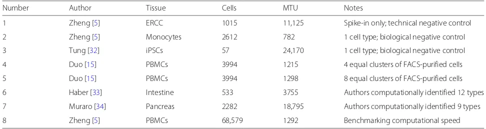
We used 9 public UMI count datasets to benchmark our

methods (Table 1). The first dataset was a highly

con-trolled experiment specifically designed to understand the technical variability. No actual cells were used to gener-ate this dataset. Instead, each droplet received the same ratio of 92 synthetic spike-in RNA molecules from Exter-nal RNA Controls Consortium (ERCC). We refer to this dataset as thetechnical replicates negative controlas there is no biological variability whatsoever, and in principle, each expression profile should be the same.

The second and third datasets contained cells from homogeneous populations purified using fluorescence-activated cell sorting (FACS). We refer to these datasets as biological replicates negative controls. Because these cells were all the same type, we did not expect to observe any significant differences in unsupervised

Table 1Single cell RNA-Seq datasets used

Number Author Tissue Cells MTU Notes

1 Zheng [5] ERCC 1015 11,125 Spike-in only; technical negative control

2 Zheng [5] Monocytes 2612 782 1 cell type; biological negative control

3 Tung [32] iPSCs 57 24,170 1 cell type; biological negative control

4 Duo [15] PBMCs 3994 1215 4 equal clusters of FACS-purified cells

5 Duo [15] PBMCs 3994 1298 8 equal clusters of FACS-purified cells

6 Haber [33] Intestine 533 3755 Authors computationally identified 12 types

7 Muraro [34] Pancreas 2282 18,795 Authors computationally identified 9 types

8 Zheng [5] PBMCs 68,579 1292 Benchmarking computational speed

Species: allH. sapiensexcept Haber (M. musculus). Protocols: all 10×except Muraro (CEL-Seq2) and Tung (SMARTer).MTUmedian total UMI count.iPSCsinduced pluripotent stem cells

UMI counts, while the SMARTer Tung data had high counts.

The fourth and fifth datasets were created by [15]. The authors allocated FACS-purified peripheral blood

mononuclear cells (PBMCs) from 10× data [5] equally

into four (Zheng 4eq dataset) and eight (Zheng 8eq dataset) clusters, respectively. In these positive control datasets, the cluster identity of all cells was assigned inde-pendently of gene expression (using FACS), so they served as the ground truth labels.

The sixth and seventh datasets contained a wider variety of cell types. However, the cluster identities were deter-mined computationally by the original authors’ unsuper-vised analyses and could not serve as a ground truth. The

10×Haber intestinal dataset had low total UMI counts,

while the CEL-Seq2 Muraro pancreas dataset had high counts.

The final Zheng dataset consisted of a larger number of unsorted PBMCs and was used to compare computa-tional speed of different dimension reduction algorithms. We refer to it as the PBMC 68K dataset.

UMI count distribution differs from reads

To illustrate the marked difference between UMI count distributions and read count distributions, we created histograms from individual genes and spike-ins of the negative control data. Here, the UMI counts are the com-putationally de-duplicated versions of the read counts; both measurements are from the same experiment, so no differences are due to technical or biological variation. The results suggest that while read counts appear zero-inflated and multimodal, UMI counts fol-low a discrete distribution with no zero inflation (Additional file1: Figure S1). The apparent zero inflation in read counts is a result of PCR duplicates.

Multinomial sampling distribution for UMI counts

Consider a single cell i containing ti total mRNA

tran-scripts. Letnibe the total number of UMIs for the same

cell. When the cell is processed by a scRNA-Seq proto-col, it is lysed, then some fraction of the transcripts are captured by beads within the droplets. A series of com-plex biochemical reactions occur, including attachment of barcodes and UMIs, and reverse transcription of the cap-tured mRNA to a cDNA molecule. Finally, the cDNA is sequenced, and PCR duplicates are removed to generate the UMI counts [5]. In each of these stages, some frac-tion of the molecules from the previous stage are lost [5,7,32]. In particular, reverse transcriptase is an ineffi-cient and error-prone enzyme [35]. Therefore, the number of UMI counts representing the cell is much less than the number of transcripts in the original cell (ni ti).

Specifically,nitypically ranges from 1000−10, 000 while

ti is estimated to be approximately 200,000 for a typical

mammalian cell [36]. Furthermore, which molecules are selected and successfully become UMIs is a random pro-cess. Letxijbe the true number of mRNA transcripts of

gene j in celli, andyij be the UMI count for the same

gene and cell. We define therelative abundanceπijas the

true number of mRNA transcripts represented by genej

in cellidivided by the total number of mRNA transcripts in celli. Relative abundance is given byπij =xij/tiwhere

total transcripts ti = jxij. Since ni ti, there is a

“competition to be counted” [37]; genes with large relative abundanceπijin the original cell are more likely to have

nonzero UMI counts, but genes with small relative abun-dances may be observed with UMI counts of exact zeros. The UMI countsyijare a multinomial sample of the true

biological countsxij, containing only relative information

about expression patterns in the cell [37,38].

The multinomial distribution can be approximated by independent Poisson distributions and overdispersed (Dirichlet) multinomials by independent negative bino-mial distributions. These approximations are useful for computational tractability. Details are provided in the “Methods” section.

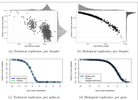
of zeros in a sample (cell or droplet) is inversely related to the total number of UMIs in that sample. Second, the probability of an endogenous gene or ERCC spike-in having zero counts is a decreasing function of its mean expression (equations provided in the “Methods” section). Both of these predictions were validated by the negative control data (Fig.1). In particular, the empirical probabil-ity of a gene being zero across droplets was well calibrated to the theoretical prediction based on the multinomial model. This also demonstrates that UMI counts are not zero inflated , consistent with [29].

To further validate the multinomial model, we assessed goodness-of-fit of seven possible null distributions to both the Tung and Zheng monocytes negative control datasets (Additional file1: Figure S2). When applied to UMI counts, the multinomial, Dirichlet-multinomial, and Poisson (as approximation to multinomial) distributions

fit best. When applied to read counts, the zero-inflated lognormal was the best fitting distribution followed by the Dirichlet-multinomial.

These results are consistent with [39], which also found that the relationship between average expression and zero probability follows the theoretical curve predicted by a Poisson model using negative control data processed with Indrop [4] and Dropseq [3] protocols. These are droplet protocols with typically low counts. It has been argued that the Poisson model is insufficient to describe the sam-pling distribution of genes with high counts and the neg-ative binomial model is more appropriate [11]. The Tung dataset contained high counts, and we nevertheless found the Poisson gave a better fit than the negative binomial. However, the difference was not dramatic, so our results do not preclude the negative binomial as a reasonable sampling distribution for UMI counts. Taken together,

these results suggest our data-generating mechanism is an accurate model of technical noise in real data.

Normalization and log transformation distorts UMI data Standard scRNA-Seq analysis involves normalizing raw counts using size factors, applying a log transformation with a pseudocount, and then centering and scaling each gene before dimension reduction. The most popular nor-malization is counts per million (CPM). The CPM are defined as(yij/ni)×106(i.e., the size factor isni/106). This

is equivalent to the maximum likelihood estimator (MLE) for relative abundanceπˆijmultiplied by 106. The log-CPM

are then log₂(c+ ˆπij106) = log2(π˜ij)+ C, where π˜ij is

a maximum a posteriori estimator (MAP) forπij

(math-ematical justification and interpretation of this approach provided in the “Methods” section). The additive constant Cis irrelevant if data are centered for each gene after log transformation, as is common practice. Thus, normaliza-tion of raw counts is equivalent to using MLEs or MAP estimators of the relative abundances.

Log transformation of MLEs is not possible for UMI counts due to exact zeros, while log transformation of MAP estimators of πij systematically distorts the

differ-ences between zero and nonzero UMI counts, depending

on the arbitrary pseudocount c(derivations provided in

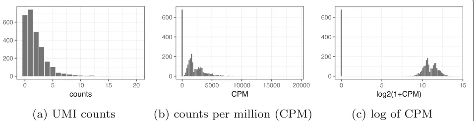
the “Methods” section). To illustrate this phenomenon, we examined the distribution of an illustrative gene before and after the log transform with varying normal-izations using the biological replicates negative control data (Fig.2). Consistent with our theoretical predictions, this artificially caused the distribution to appear zero inflated and exaggerated differences between cells based on whether the count was zero or nonzero.

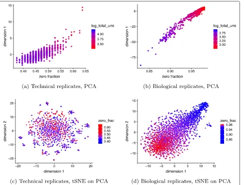
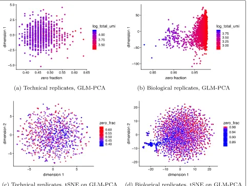
Focusing on the entire negative control datasets, we applied PCA to log-CPM values. We observed a strong

correlation (r = 0.8 for technical and r = 0.98 for

monocytes biological replicates) between the first princi-pal component (PC) and the fraction of zeros, consistent

with [30]. Application of PCA to CPM values without log

transform reduced this correlation tor = 0.1 for

tech-nical and r = 0.7 for monocytes biological replicates.

Additionally, the first PC of log-CPM correlated with the log of total UMI, which is consistent with the multinomial model (Fig.3). Note that in datasets with strong biological variability, the nuisance variation from zero fraction and total counts could appear in secondary PCs rather than the first PC, but it would still confound downstream anal-yses. Based on these results, the log transformation is not necessary and in fact detrimental for the analysis of UMI counts. The benefits of avoiding normalization by instead directly modeling raw counts have been demonstrated in the context of differential expression [40]. Where normal-ization is unavoidable, we propose the use of approximate multinomial deviance residuals (defined in the “Residuals andz-scores” section) instead of log-transformed CPM.

Zero inflation is an artifact of log normalization

To see how normalization and log transformation intro-duce the appearance of zero inflation, consider the follow-ing example. Letyijbe the observed UMI counts following

a multinomial distribution with sizeni for each cell and

relative abundanceπjfor each gene, constant across cells.

Focusing on a single genej,yij follows a binomial

distri-bution with parametersniandpj. Assumeπj= 10−4and

theni range from 1000−3000, which is consistent with

the biological replicates negative control data (Fig.1and Additional file1: Figure S1). Under this assumption, we expect to see about 74–90% zeros, 22–30% ones, and less than 4% values above one. However, notice that after nor-malization to CPM and log transformation, all the zeros remain log 2(1+0) = 0, yet the ones turn into values ranging from log₂(1+1/3000×106) = log₂(334) ≈ 8.4 to log₂(1001) ≈ 10. The few values that are 2 will have values ranging from log₂(668) ≈ 9.4 to log₂(2001) ≈ 11. The large, artificial gap between zero and nonzero val-ues makes the log-normalized data appear zero-inflated

Fig. 2Example of how current approaches to normalization and transformation artificially distort differences between zero and nonzero counts.

Fig. 3Current approaches to normalization and transformation induce variability in the fraction of zeros across cells to become the largest source of variability which in turn biases clustering algorithms to produce false-positive results based on distorted latent factors.aFirst principal component (PC) from the technical replicates dataset plotted against fraction of zeros for each cell. A red to blue color scale represents total UMIs per cell.bAsa

but for the monocytes biological replicates data.cUsing the technical replicates, we applied t-distributed stochastic neighbor embedding (tSNE) with perplexity 30 to the top 50 PCs computed from log-CPM. The first 2 tSNE dimensions are shown with a blue to red color scale representing the fraction of zeros.dAscbut for the biological replicates data. Here, we do not expect to find differences, yet we see distorted latent factors being driven by the total UMIs. PCA was applied to 5000 random genes

(Fig. 2). The variability in CPM values across cells is

almost completely driven by the variability inni. Indeed, it

shows up as the primary source of variation in PCA plots (Fig.3).

Generalized PCA for dimension reduction of sparse counts While PCA is a popular dimension reduction method, it is implicitly based on Euclidean distance, which corresponds to maximizing a Gaussian likelihood. Since UMI counts are not normally distributed, even when normalized and log transformed, this distance metric is inappropriate [41], causing PCA to produce distorted latent factors (Fig.3). We propose the use of PCA for generalized linear models (GLMs) [31] or GLM-PCA as a more appropriate alterna-tive. The GLM-PCA framework allows for a wide variety

section). We implemented both negative binomial and Poisson GLM-PCA, but we focused primarily on the latter in our assessments for simplicity of exposition. Intuitively, using Poisson instead of negative binomial implies, we assume the biological variability is captured by the fac-tor model and the unwanted biological variability is small relative to the sampling variability. Our implementation also allows the user to adjust for gene-specific or cell-specific covariates (such as batch labels) as part of the overall model.

We ran Poisson GLM-PCA on the technical and bio-logical (monocytes) replicates negative control datasets and found it removed the spurious correlation between the first dimension and the total UMIs and fraction of

zeros (Fig.4). To examine GLM-PCA as a visualization

tool, we ran Poisson and negative binomial GLM-PCA

along with competing methods on the 2 ground truth datasets (Additional file1: Figure S3). For the Zheng 4eq dataset, we directly reduced to 2 dimensions. For the Zheng 8eq dataset, we reduced to 15 dimensions then applied UMAP [42]. While all methods effectively sep-arated T cells from other PBMCs, GLM-PCA methods also separated memory and naive cytotoxic cells from the other subtypes of T cells. This separation was not visible with PCA on log-CPM. Computational speed is discussed in the “Computational efficiency of multinomial models” section.

Deviance residuals provide fast approximation to GLM-PCA One disadvantage of GLM-PCA is it depends on an iter-ative algorithm to obtain estimates for the latent factors and is at least ten times slower than PCA. We therefore

propose a fast approximation to GLM-PCA. When using PCA a common first step is to center and scale the data for each gene as z-scores. This is equivalent to the fol-lowing procedure. First, specify a null model of constant gene expression across cells, assuming a normal distri-bution. Next, find the MLEs of its parameters for each gene (the mean and variance). Finally, compute the resid-uals of the model as thez-scores (derivation provided in the “Methods” section). The fact that scRNA-Seq data are skewed, discrete, and possessing many zeros suggests the normality assumption may be inappropriate. Further, using z-scores does not account for variability in total UMIs across cells. Instead, we propose to replace the nor-mal null model with a multinomial null model as a better match to the data-generating mechanism. The analogs to z-scores under this model are called deviance and Pear-son residuals. Mathematical formulae are presented in the “Methods” section. The use of multinomial residu-als enables a fast transformation similar toz-scores that avoids difficulties of normalization and log transformation by directly modeling counts. Additionally, this framework allows straightforward adjustment for covariates such as cell cycle signatures or batch labels. In an illustrative sim-ulation (details in the “Residuals andz-scores” section), residual approximations to GLM-PCA lost accuracy in the presence of strong batch effects, but still outperformed the traditional PCA (Additional file1: Figure S4). System-atic comparisons on ground truth data are provided in the “Multinomial models improve unsupervised clustering” section.

Computational efficiency of multinomial models

We measured time to convergence for reduction to two latent dimensions of GLM-PCA, ZINB-WAVE, PCA on log-CPM, PCA on deviance residuals, and PCA on Pear-son residuals. Using the top 600 informative genes, we subsampled the PBMC 68K dataset to 680, 6800, and 68,000 cells. All methods scaled approximately linearly with increasing the numbers of cells, but GLM-PCA was 23–63 times faster than ZINB-WAVE across sample sizes (Additional file1: Figure S5). Specifically, GLM-PCA pro-cessed 68,000 cells in less than 7 min. The deviance and Pearson residuals methods exhibited speeds compara-ble to PCA: 9–26 times faster than GLM-PCA. We also timed dimension reduction of the 8eq dataset (3994 cells) from 1500 informative genes to 10 latent dimensions. PCA (with either log-CPM, deviance, or Pearson residu-als) took 7 s, GLM-PCA took 4.7 min, and ZINB-WAVE took 86.6 min.

Feature selection using deviance

Feature selection, or identification of informative genes, may be accomplished by ranking genes using thedeviance, which quantifies how well each gene fits a null model

of constant expression across cells. Unlike the competing highly variable or highly expressed genes methods, which are sensitive to normalization, ranking genes by deviance operates on raw UMI counts. An approximate multino-mial deviance statistic can be computed in closed form (formula provided in the “Methods” section).

We compared gene ranks for all three feature selection methods (deviance, highly expressed, and highly variable

genes) on the 8eq dataset (Table1). We found a strong

concordance between highly deviant genes and highly expressed genes (Spearman’s rank correlationr=0.9987), while highly variable genes correlated weakly with both high expression (r=0.3835) and deviance (r=0.3738).

Choosing informative genes by high expression alone would be ineffective if a gene had high but constant expression across cells. To ensure the deviance criterion did not identify such genes, we created a simulation with three types of genes: lowly expressed, high but constantly expressed, and high and variably expressed. Deviance preferentially selected high and variably expressed genes while filtering by highly expressed genes identified the constantly expressed genes before the variably expressed (Additional file1: Figure S6, Table S1). Furthermore, an examination of the top 1000 genes by each criteria on the Muraro dataset showed that deviance did not identify the same set of genes as highly expressed genes (Addi-tional file 1: Figure S7, Table S2). Empirically, deviance seems to select genes that are both highly expressed and highly variable, which provides a rigorous justification for a common practice.

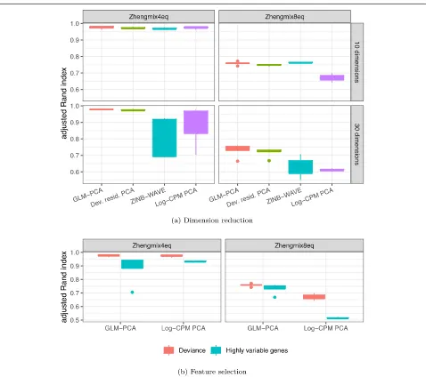
Multinomial models improve unsupervised clustering Dimension reduction with GLM-PCA or its fast multino-mial residuals approximation improved clustering perfor-mance over competing methods (Fig.5a, Additional file1: Figure S8a). Feature selection by multinomial deviance was superior to highly variable genes (Fig.5b).

Using the two ground truth datasets described under the “Datasets” section, we systematically compared the clustering performance of all combinations of previously described methods for normalization, feature selection, and dimension reduction. In addition, we compared against ZINB-WAVE since it also avoids requiring the user to pre-process and normalize the UMI count data (e.g., log transformation of CPM) and accounts for vary-ing total UMIs across cells [28]. After obtainvary-ing latent

factors, we used Seurat’s Louvain implementation and

Fig. 5Dimension reduction with GLM-PCA and feature selection using deviance improves Seurat clustering performance. Each column represents a different ground truth dataset from [15].aComparison of dimension reduction methods based on the top 1500 informative genes identified by approximate multinomial deviance. The Poisson approximation to the multinomial was used for GLM-PCA. Dev. resid. PCA, PCA on approximate multinomial deviance residuals.bComparison of feature selection methods. The top 1500 genes identified by deviance and highly variable genes were passed to 2 different dimension reduction methods: GLM-PCA and PCA on log-transformed CPM. Only the results with the number of clusters within 25% of the true number are presented

their extensive benchmarking (details are provided in the “Methods” section).

We compared the Seurat clustering performance of GLM-PCA (with Poisson approximation to multinomial) to running PCA on deviance residuals, which adhere more closely to the normal distribution than log-CPM. We found both of these approximate multinomial methods gave similar results on the 4eq dataset and outperformed

PCA on log-CPMz-scores. However, GLM-PCA

outper-formed the residuals method on the 8eq dataset. Also, performance on ZINB-WAVE factors degraded when the number of latent dimensions increased from 10 to

30, whereas GLM-PCA and its fast approximation with deviance residuals were robust to this change (Fig. 5a). GLM-PCA and its residual approximations produced better cluster separation than PCA or ZINB-WAVE, even in scenarios where all methods had similar accu-racy (Additional file 1: Figure S8a). The performance of Pearson residuals was similar to that of deviance residuals (Additional file1: Figure S9, S10).

Focusing on feature selection methods, deviance

had higher accuracy than highly variable genes

across both datasets and across dimension reduction

led to similar clustering performance as deviance

(Additional file 1: Figure S9), because both criteria

identified strongly overlapping gene lists for these data. The combination of feature selection with deviance and dimension reduction with GLM-PCA also improved

clustering performance whenk-means was used in place

of Seurat (Additional file1: Figure S11). A complete table of results is publicly available (see the “Availability of data and materials” section).

Finally, we examined the clustering performance of competing dimension reduction methods on two

pub-lic datasets with more complex subtypes (Table 1). The

10× Haber dataset [33] was annotated with 12 types

of enteroendocrine cells from the intestine. The CEL-Seq2 Muraro dataset [34] was annotated with 9 types of pancreatic cells. Since these cluster labels were com-putationally derived, they did not constitute a ground truth comparison. Nevertheless, GLM-PCA had the clos-est concordance with the original authors’ annotation in both datasets (Additional file1: Tables S3, S4).

Conclusions

We have outlined a statistical framework for analysis of scRNA-Seq data with UMI counts based on a multino-mial model, providing effective and simple to compute methods for feature selection and dimension reduction. We found that UMI count distributions differ dramatically from read counts, are well-described by a multinomial distribution, and are not zero inflated. Log transforma-tion of normalized UMI counts is detrimental, because it artificially exaggerates the differences between zeros and all other values. For feature selection, or identifica-tion of informative genes, deviance is a more effective criterion than highly variable genes. Dimension reduction via GLM-PCA, or its fast approximation using residu-als from a multinomial model, leads to better clustering

performance than PCA onz-scores of log-CPM.

Although our methods were inspired by scRNA-Seq UMI counts, they may be useful for a wider array of data sources. Any high dimensional, sparse dataset where samples contain only relative information in the form of counts may conceivably be modeled by the multinomial distribution. Under such scenarios, our methods are likely to be more effective than applying log transformations and standard PCA. A possible example is microbiome data.

We have not addressed major topics in the scRNA-Seq literature such as pseudotime inference [44], differential expression [45], and spatial analysis [46]. However, the sta-tistical ideas outlined here can also be used to improve methods in these more specialized types of analyses.

Our results have focused on (generalized) linear mod-els for simplicity of exposition. Recently, several promis-ing nonlinear dimension reductions for scRNA-Seq have been proposed. The variational autoencoder (VAE, a type

of neural network) method scVI [47] utilizes a negative binomial likelihood in the decoder, while the encoder relies on log-normalized input data for numerical stability. The Gaussian process method tGPLVM [48] models log-transformed counts. In both cases, we suggest replac-ing log-transformed values with deviance residuals to improve performance. Nonlinear dimension reduction methods may also depend on feature selection to reduce memory consumption and speed computation; here, our deviance method may be utilized as an alternative to high variability for screening informative genes.

Methods

Multinomial model for scRNA-Seq

Letyijbe the observed UMI counts for cell or dropletiand

gene or spike-inj. Letni=jyijbe the total UMIs in the

sample, andπijbe the unknown true relative abundance of

genejin celli. The random vectoryi=(yi1,. . .,yiJ)with

constraint_jyij = nifollows a multinomial distribution

with densit function:

f(yi)=

ni

yi1,. . .,yiJ _j π yij

ij

Focusing on a single gene jat a time, the marginal dis-tribution of yij is binomial with parameters ni and πij.

The marginal mean is E[yij]= niπij = μij, the marginal

variance is var[yij]= niπij(1− πij) = μij − _n1_iμ2_ij, and

the marginal probability of a zero count is(1−πij)ni =

1−μij_n

i ni

. The correlation between two genesj,kis:

cor[yij,yik]=

−√πijπik

(1−πij)(1−πik)

The correlation is induced by the sum to ni constraint.

As an extreme example, if there are only two genes (J =

2), increasing the count of the first gene automatically reduces the count of the second gene since they must add

up toni under multinomial sampling. This means when

J=2, there is a perfect anti-correlation between the gene counts which has nothing to do with biology. More gen-erally, when either J or ni is small, gene counts will be

negatively correlated independent of biological gene-gene correlations, and it is not possible to analyze the data on a gene-by-gene basis (for example, by ranking and filtering genes for feature selection). Rather, comparisons are only possible between pairwise ratios of gene expression values [49]. Yet, this type of analysis is difficult to interpret and computationally expensive for large numbers of genes (i.e., in high dimensions). Fortunately, under certain assump-tions, more tractable approximations may be substituted for the true multinomial distribution.

First, note that if correlation is ignored, the multinomial

may be approximated by J-independent binomial

if allπij are very small, which is likely to be satisfied for

scRNA-Seq if the number of genesJis large, and no sin-gle gene constitutes the majority of mRNAs in the cell. If ni is large and πij is small, each binomial

distribu-tion can be further approximated by a Poisson with mean niπij. Alternatively, the multinomial can be constructed

by drawingJ-independent Poisson random variables and

conditioning on their sum. IfJandniare large, the

differ-ence between the conditional, multinomial distribution, and the independent Poissons becomes negligible. Since in practiceni is large, the Poisson approximation to the

multinomial may be reasonable [50–53].

The multinomial model does not account for biologi-cal variability. As a result, an overdispersed version of the multinomial model may be necessary. This can be accom-modated with the Dirichlet-multinomial distribution. Let

yi be distributed as a multinomial conditional on the

rel-ative abundance parameter vectorπi = (πi1,. . .,πiJ).

If πi is itself a random variable with symmetric

Dirich-let distribution having shape parameter α, the marginal distribution ofyi is Dirichlet-multinomial. This

distribu-tion can itself be approximated by independent negative binomials. First, note that a symmetric Dirichlet

ran-dom vector can be constructed by drawingJ-independent

gamma variates with shape parameterαand dividing by

their sum. Suppose (as above) we approximate the condi-tional multinomial distribution ofyi such thatyijfollows

an approximate Poisson distribution with meanniπij. Let

λijbe a collection of non-negative random variables such

that πij = λij

jλij. We require that πi follows a symmet-ric Disymmet-richlet, which is accomplished by havingλij follow

independent gamma distributions with shapeαand mean

ni/J. This impliesjλij follows a gamma with shapeJα

and meanni. AsJ → ∞, this distribution converges to

a point mass at ni, so for large J (satisfied by

scRNA-Seq), _jλij ≈ ni. This implies that yij approximately

follows a conditional Poisson distribution with meanλij,

where λij is itself a gamma random variable with mean

ni/J and shapeα. If we then integrate outλij we obtain

the marginal distribution ofyijas negative binomial with

shapeαand meanni/J. Hence a negative binomial model

for count data may be regarded as an approximation to an overdispersed Dirichlet-multinomial model.

Parameter estimation with multinomial models (and their binomial or Poisson approximations) is straight-forward. First, suppose we observe replicate samples yi,

i = 1,. . .,I from the same underlying population of molecules, where the relative abundance of genejisπj.

This is a null model because it assumes each gene has a constant expected expression level, and there is no biolog-ical variation across samples. Regardless of whether one assumes a multinomial, binomial, or Poisson model, the maximum likelihood estimator (MLE) ofπjisπˆj =

iyij

ini

whereniis the total count of samplei. In the more

real-istic case that relative abundancesπijof genes vary across

samples, the MLE isπˆij= y_nij_i.

An alternative to the MLE is the maximum a posteri-ori (MAP) estimator. Suppose a symmetric Dirichlet prior

with concentration parameter αi is combined with the

multinomial likelihood for celli. The MAP estimator for

πijis given by:

˜

πij= αi+

yij

Jαi+ni =

wi

1

J +(1−wi)πˆij

where wi = Jαi/(Jαi + ni), showing that the MAP is

a weighted average of the prior mean that all genes are equally expressed (1/J) and the MLE (πˆij). Compared to

the MLE, the MAP biases the estimate toward the prior where all genes have the same expression. Larger values of

αi introduce more bias, whileαi → 0 leads to the MLE.

Ifαi > 0, the smallest possible value ofπ˜ij isαi/(Jαi+

ni)rather than zero for the MLE. When there are many

zeros in the data, MAP can stabilize relative abundance estimates at the cost of introducing bias.

Mathematics of distortion from log-normalizing UMIs Suppose the true counts in celliare given byxijfor genes

j = 1,. . .,J. Some of these may be zero, if a gene is not turned on in the cell. Knowingxijis equivalent to

know-ing the total number of transcripts ti = jxij and the

relative proportions of each geneπij, sincexij=tiπij. The

total number of UMI countsni = jyij does not

esti-mateti. However, under multinomial sampling, the UMI

relative abundancesπˆij = y_nij_i are MLEs for the true

pro-portions πij. Note that it is possible that πˆij = 0 even

thoughπij > 0. Becausejπˆij = 1 regardless ofni, the

use of multinomial MLEs is equivalent to the widespread practice of normalizing each cell by the total counts. Furthermore, the use of size factorssi = ni/mleads to

ˆ

πij×m(ifm=106, this is CPM).

Traditional bulk RNA-Seq experiments measured gene expression in read counts of many cells per sample rather than UMI counts of single cells. Gene counts from bulk RNA-Seq could thus range over several orders of mag-nitude. To facilitate comparison of these large numbers, many bulk RNA-Seq methods have relied on a logarithm transformation. This enables interpretation of differences in normalized counts as fold changes on a relative scale. Also, for count data, the variance of each gene is a function of its mean, and log transformation can help to prevent highly expressed outlier genes from overwhelming down-stream analyses. Prior to the use of UMIs, scRNA-Seq experiments also produced read counts with wide ranging values, and a log transform was again employed. However, with single cell data, more than 90% of the genes might

be observed as exact zeros, and log(0) = −∞ which is

numbers of zeros, but do not contain very large counts since PCR duplicates have been removed. Nevertheless, log transformation has been commonly used with UMI data as well.

The current standard is to transform the UMI counts as log₂(c+ ˆπij ×m) wherec is a pseudocount to avoid

taking the log of zero, and typicallyc = 1. As before,m is some constant such as 106for CPM (see also [54] for an alternative). Finally, the data are centered and scaled so that the mean of each gene across cells is 0, and the stan-dard deviation is 1. This stanstan-dardization of the data causes any subsequent computation of distances or dimension reduction to be invariant to constant additive or multi-plicative scaling. For example, under Manhattan distance, d(x+c,y+c) = |x+c−(y+c)| = |x−y| =d(x,y). In particular, using size factors such as CPM instead of rel-ative abundances leads to a rescaling of the pseudocount, and use of any pseudocount is equivalent to replacing the

MLE with the MAP estimator. Let k = c/mand αi =

kni. Then, the weight term in the MAP formula becomes

wi =Jk/(1+Jk) = wwhich is constant across all cellsi.

FurthermoreJk=w/(1−w), showing that:

log₂(c+ ˆπij×m)=log₂(k+ ˆπij)+log₂(m)

=log₂

w

1−w

1

J + ˆπij

+log₂(m)

=log₂

w1

J +(1−w)πijˆ

−log₂(1−w)+log₂(m)

=log₂(πij)˜ +C

Where C is a global constant that does not vary across

cells or genes. For illustration, ifc=1 andm=106, this is equivalent to assuming a prior where all genes are equally expressed and for celli, a weight ofw=J/(106+J)is given to the prior relative to the MLE. Since the number of genes Jis on the order of 104, we havew≈.01. The prior sample size for celliisJαi = 10−6Jni ≈ .01×niwhereni is the

data sample size. The standard transformation is therefore equivalent to using a weak prior to obtain a MAP estimate of the relative abundances, then log transforming before dimension reduction.

In most scRNA-Seq datasets, the total number of UMIs ni for some cells may be significantly less than the

con-stantm. For these cells, the size factorssi =ni/mare less

than 1. Therefore, after normalization (dividing by size factor), the counts are scaled up to match the target size ofm. Due to the discreteness of counts, this introduces a bias after log transformation, if the pseudocount is small (or equivalently, ifmis large). For example, letc= 1 and m=106(CPM). Ifni =104for a particular cell, we have

si =.01. A raw count ofyij= 1 for this cell is normalized

to 1/.01 = 100 and transformed to log₂(1+100) = 6.7. For this cell, on the log scale, there cannot be any values between 0 and 6.7 because fractional UMI counts cannot

be observed and log₂(1 +0) = 0. Small pseudocounts

and small size factors combined with log transform arbi-trarily exaggerate the difference between a zero count and a small nonzero count. As previously shown, this sce-nario is equivalent to using MAP estimation of πij with

a weak prior. To combat this distortion, one may attempt to strengthen the prior to regularizeπ˜ijestimation at the

cost of additional bias, as advocated by [21]. An extreme

case occurs whenc=1 andm= 1. Here, the prior

sam-ple size isJni, so almost all the weight is on the prior. The

transform is then log₂(1+ ˆπij). But this function is

approx-imately linear on the domain 0≤ ˆπij≤1. After centering

and scaling, a linear transformation is vacuous.

To summarize, log transformation with a weak prior (small size factor, such as CPM) introduces strong arti-ficial distortion between zeros and nonzeros, while log tranformation with a strong prior (large size factor) is roughly equivalent to not log transforming the data.

Generalized PCA

PCA minimizes the mean squared error (MSE) between the data and a low-rank representation, or embedding. Let yijbe the raw counts andzijbe the normalized and

trans-formed version ofyijsuch as centered and scaled log-CPM

(z-scores). The PCA objective function is:

min

u,v i,j

(zij− uivj)2

where ui,vj ∈ RL for i = 1,. . .,I, j = 1,. . .,J. The

ui are called factors or principal components, and thevj

are called loadings. The number of latent dimensions L

controls the complexity of the model. Minimization of the MSE is equivalent to minimizing the Euclidean dis-tance metric between the embedding and the data. It is also equivalent to maximizing the likelihood of a Gaussian model:

zij∼N

u_ivj,σ2

If we replace the Gaussian model with a Poisson, which approximates the multinomial, we can directly model the UMI counts as:

yij∼Poi

niexp{uivj}

or alternatively, in the case of overdispersion, we may approximate the Dirichlet-multinomial using a negative binomial likelihood:

yij∼NB

niexp{uivj}; φj

We define the linear predictor as ηij = logni + u_ivj.

It is clear that the mean μij = eη_ij appears in both the

Poisson and negative binomial model statements, showing that the latent factors interact with the data only through the mean. We may then estimate ui andvj (and φj) by

L2 penalty to large parameter values improves numeri-cal stability). A link function must be used since ui and

vjare real valued whereas the mean of a Poisson or

nega-tive binomial must be posinega-tive. The total UMIsniterm is

used as an offset since no normalization has taken place; alternative size factorssi such as those from scran [20]

could be used in place ofni. If the first element of each

ui is constrained to equal 1, this induces a gene-specific

intercept term in the first position of eachvj, which is

analogous to centering. Otherwise, the model is very sim-ilar to that of PCA; it is simply optimizing a different objective function. Unfortunately, MLEs foruiandvj

can-not be expressed in closed form, so an iterative Fisher scoring procedure is necessary. We refer to this model as GLM-PCA [55]. Just as PCA minimizes MSE, GLM-PCA

minimizes a generalization of MSE called the deviance

[56]. While generalized PCA was originally proposed by [31] (see also [57] and [58]), our implementation is novel in that it allows for intercept terms, offsets, overdisper-sion, and non-canonical link functions. We also use a blockwise update for optimization which we found to be more numerically stable than that of [31]; we iterate over

latent dimensions l rather than rows or columns. This

technique is inspired by non-negative matrix factorization algorithms such as hierarchical alternating least squares and rank-one residue iteration, see [59] for a review.

As an illustration, consider GLM-PCA with the Poisson approximation to a multinomial likelihood. The objective function to be minimized is simply the overall deviance:

D=

i,j

yijlog

yij

μij

−(yij−μij)

logμij=ηij=logsi+ uivj=logsi+vj1+

L

l=2

uilvjl

wheresiis a fixed size factor such as the total number of

UMIs (ni). The optimization proceeds by taking

deriva-tives with respect to the unknown parameters: vj1 is a

gene-specific intercept term, and the remaininguilandvjl

are the latent factors.

The GLM-PCA method is most concordant to the data-generating mechanism since all aspects of the pipeline are integrated into a coherent model rather than being dealt with through sequential normalizations and transforma-tions. The interpretation of the ui andvj vectors is the

same as in PCA. For example, suppose we set the num-ber of latent dimensions to 2 (i.e.,L = 3 to account for the intercept). We can plotui2on the horizontal axis and

ui3on the vertical axis for each cellito visualize the

rela-tionships between cells such as gradients or clusters. In this way, theuiandvjcapture biological variability such as

differentially expressed genes.

Residuals andz-scores

Just as mean squared error can be computed by taking the sum of squared residuals under a Gaussian likelihood, the deviance is equal to the sum of squareddeviance resid-uals [56]. Since deviance residuals are not well-defined for the multinomial distribution, we adopt the binomial approximation. The deviance residual for genejin celliis given by:

r(_ijd)=sign(yij− ˆμij)

2yijlog

yij

ˆ

μij +

2(ni−yij)log

ni−yij

ni− ˆμij

where under the null model of constant gene expression across cells,μˆij = niπˆj. The deviance residuals are the

result of regressing away this null model. An alternative to deviance residuals is the Pearson residual, which is sim-ply the difference in observed and expected values scaled by an estimate of the standard deviation. For the binomial, this is:

r(_ijp)= yij− ˆμij ˆ

μij−_n1_iμˆ2_ij

According to the theory of generalized linear models (GLM), both types of residuals follow approximately a normal distribution with mean zero if the null model is correct [56]. Deviance residuals tend to be more symmet-ric than Pearson residuals. In practice, the residuals may not have mean exactly equal to zero, and may be stan-dardized by scaling their gene-specific standard deviation just as in the Gaussian case. Recently, Pearson residuals based on a negative binomial null model have also been independently proposed as the sctransform method [60].

The z-score is simply the Pearson residual where we replace the multinomial likelihood with a Gaussian (nor-mal) likelihood and use normalized values instead of raw

UMI counts. Let qij be the normalized (possibly

log-transformed) expression of genejin celliwithout center-ing and scalcenter-ing. The null model is that the expression of the gene is constant across all cells:

qij∼N

μj, σj2

The MLEs areμˆj = 1_Iiqij,σˆ_j2 = 1_Ii(qij− ˆμj)2, and

thez-scores equal the Pearson residualszij=(qij− ˆμj)/σˆj.

We compared the accuracy of the residuals approxi-mations by simulating 150 cells in 3 clusters of 50 cells each with 5000 genes, of which 500 were differentially expressed across clusters (informative genes). We also cre-ated 2 batches, batch 1 with total counts of 1000 and batch 2 with total counts of 2000. Each cluster had an equal number of cells in the 2 batches. We then ran

GLM-PCA on the raw counts, GLM-PCA on log2(1+ CPM), PCA

on deviance residuals, and PCA on Pearson residuals with

Feature selection using deviance

Genes with constant expression across cells are not infor-mative. Such genes may be described by the multinomial null model whereπij = πj. Goodness of fit to a

multino-mial distribution can be quantified using deviance, which is twice the difference in log-likelihoods comparing a sat-urated model to a fitted model. The multinomial deviance is a joint deviance across all genes,and for this reason is not helpful for screening informative genes. Instead, one may use the binomial deviance as an approximation:

Dj=2 i

yijlog

yij

niπˆj +(

ni−yij)log (

ni−yij)

ni(1− ˆπj)

A large deviance value indicates the model in question provides a poor fit. Those genes with biological variation across cells will be poorly fit by the null model and will have the largest deviances. By ranking genes according to their deviances, one may thus obtain highly deviant genes as an alternative to highly variable or highly expressed genes.

Systematic comparison of methods

We considered combinations of the following methods and parameter settings, following [15]. Italics indicate methods proposed in this manuscript. Feature selec-tion: highly expressed genes, highly variable genes, and highly deviant genes. We did not compare against highly dropout genes because [15] found this method to have poor downstream clustering performance for UMI counts and it is not as widely used in the literature. The num-bers of genes are 60, 300, 1500. Normalization, trans-formation, and dimension reduction: PCA on log-CPM z-scores, ZINB-WAVE [28], PCA on deviance residu-als, PCA on Pearson residuals, and GLM-PCA. The numbers of latent dimensions are 10 and 30.

Cluster-ing algorithms are k-means [61] and Seurat [17]. The

number of clusters is all values from 2 to 10, inclu-sive. Seurat resolutions are 0.05, 0.1, 0.2, 0.5, 0.8, 1, 1.2, 1.5, and 2.

Supplementary information

Supplementary informationaccompanies this paper at

https://doi.org/10.1186/s13059-019-1861-6.

Additional file 1: Contains supplementary figures S1–S11 and tables S1–S4.

Additional file 2: Review history.

Acknowledgements

The authors thank Keegan Korthauer, Jeff Miller, Linglin Huang, Alejandro Reyes, Yered Pita-Juarez, Mike Love, Ziyi Li, and Kelly Street for the valuable suggestions.

Review history

The review history is available as Additional file2.

Peer review information

Barbara Cheifet was the primary editor of this article and managed its peer review in collaboration with the rest of the editorial team.

Authors’ contributions

SCH, MJA, and RAI identified the problem. FWT proposed, derived, and implemented the GLM-PCA model, its fast approximation using residuals, and feature selection using deviance. SCH, MJA, and RAI provided guidance on refining the methods and evaluation strategies. FWT and RAI wrote the draft manuscript, and revisions were suggested by SCH and MJA. All authors approved the final manuscript.

Funding

FWT was supported by NIH grant T32CA009337, SCH was supported by NIH grant R00HG009007, MJA was supported by an MGH Pathology Department startup fund, and RAI was supported by Chan-Zuckerberg Initiative grant CZI 2018-183142 and NIH grants R01HG005220, R01GM083084, and P41HG004059.

Availability of data and materials

All methods and assessments described in this manuscript are publicly available athttps://github.com/willtownes/scrna2019[62]. GLM-PCA is available as an R package from CRAN (https://cran.r-project.org/web/ packages/glmpca/index.html). The source code is licensed under LGPL-3. All datasets used in the study were obtained from public sources (Table1). The three Zheng datasets (ERCCs, monocytes, and 68K PBMCs) [5] were

downloaded from https://support.10xgenomics.com/single-cell-gene-expression/datasets. The Duo datasets were obtained through the bioconductor package DuoClustering2018 [15]. The remaining three datasets had GEO accession numbers GSE77288 (Tung) [32], GSE92332 (Haber) [33], and GSE85241 (Muraro) [34].

Ethics approval and consent to participate Not applicable.

Consent for publication Not applicable.

Competing interests

The authors declare that they have no competing interests.

Author details

1_{Department of Biostatistics, Harvard University, Cambridge, MA, USA.} 2_{Present Address: Department of Computer Science, Princeton University,}

Princeton, NJ, USA.3_{Department of Biostatistics, Johns Hopkins University,} Baltimore, MD, USA.4_{Molecular Pathology Unit, Massachusetts General} Hospital, Charlestown, MA, USA.5_{Center for Cancer Research, Massachusetts} General Hospital, Charlestown, MA, USA.6_{Department of Pathology, Harvard} Medical School, Boston, MA, USA.7_{Department of Data Sciences, Dana-Farber} Cancer Institute, Boston, MA, USA.

Received: 12 March 2019 Accepted: 15 October 2019

References

1. Kalisky T, Oriel S, Bar-Lev TH, Ben-Haim N, Trink A, Wineberg Y, Kanter I, Gilad S, Pyne S. A brief review of single-cell transcriptomic technologies. Brief Funct Genom. 2018;17(1):64–76.https://doi.org/10.1093/bfgp/ elx019.

2. Svensson V, Vento-Tormo R, Teichmann SA. Exponential scaling of single-cell RNA-seq in the past decade. Nat Protoc. 2018;13(4):599–604.

https://doi.org/10.1038/nprot.2017.149.

3. Macosko EZ, Basu A, Satija R, Nemesh J, Shekhar K, Goldman M, Tirosh I, Bialas A. R, Kamitaki N, Martersteck EM, Trombetta JJ, Weitz DA, Sanes JR, Shalek AK, Regev A, McCarroll SA. Highly parallel genome-wide expression profiling of individual cells Using nanoliter droplets. Cell. 2015;161(5):1202–14.https://doi.org/10.1016/j.cell.2015.05.002. 4. Klein AM, Mazutis L, Akartuna I, Tallapragada N, Veres A, Li V, Peshkin L,

5. Zheng GXY, Terry JM, Belgrader P, Ryvkin P, Bent ZW, Wilson R, Ziraldo SB, Wheeler TD, McDermott GP, Zhu J, Gregory MT, Shuga J, Montesclaros L, Underwood JG, Masquelier DA, Nishimura SY, Schnall-Levin M, Wyatt PW, Hindson CM, Bharadwaj R, Wong A, Ness KD, Beppu LW, Deeg HJ, McFarland C, Loeb KR, Valente WJ, Ericson NG, Stevens EA, Radich JP, Mikkelsen TS, Hindson BJ, Bielas JH. Massively parallel digital transcriptional profiling of single cells. Nat Commun. 2017;8:14049.https://doi.org/10.1038/ncomms14049.

6. Dal Molin A, Di Camillo B. How to design a single-cell RNA-sequencing experiment: pitfalls, challenges and perspectives. Brief Bioinform. 2018.

https://doi.org/10.1093/bib/bby007.

7. Qiu X, Hill A, Packer J, Lin D, Ma Y-A, Trapnell C. Single-cell mRNA quantification and differential analysis with Census. Nat Methods. 2017;14(3):309–15.https://doi.org/10.1038/nmeth.4150.

8. Picelli S, Björklund ÅK, Faridani OR, Sagasser S, Winberg G, Sandberg R. Smart-seq2 for sensitive full-length transcriptome profiling in single cells. Nat Methods. 2013;10(11):1096–8.https://doi.org/10.1038/nmeth.2639. 9. Kolodziejczyk AA, Kim JK, Svensson V, Marioni JC, Teichmann SA. The

technology and biology of single-cell RNA sequencing. Mol Cell. 2015;58(4):610–20.https://doi.org/10.1016/j.molcel.2015.04.005. 10. Islam S, Zeisel A, Joost S, La Manno G, Zajac P, Kasper M, Lönnerberg P,

Linnarsson S. Quantitative single-cell RNA-seq with unique molecular identifiers. Nat Methods. 2014;11(2):163–6.https://doi.org/10.1038/ nmeth.2772.

11. Grün D, Kester L, van Oudenaarden A. Validation of noise models for single-cell transcriptomics. Nat Methods. 2014;11(6):637–40.https://doi. org/10.1038/nmeth.2930.

12. Lun ATL, McCarthy DJ, Marioni JC. A step-by-step workflow for low-level analysis of single-cell RNA-seq data with Bioconductor. F1000Research. 2016;5:2122.https://doi.org/10.12688/f1000research.9501.2. 13. McCarthy DJ, Campbell KR, Lun ATL, Wills QF. Scater: pre-processing,

quality control, normalization and visualization of single-cell RNA-seq data in R. Bioinformatics. 2017;33(8):1179–86.https://doi.org/10.1093/ bioinformatics/btw777.

14. Andrews TS, Hemberg M. Identifying cell populations with scRNASeq. Mol Asp Med. 2017.https://doi.org/10.1016/j.mam.2017.07.002. 15. Duò A, Robinson MD, Soneson C. A systematic performance evaluation

of clustering methods for single-cell RNA-seq data. F1000Research. 2018;7:1141.https://doi.org/10.12688/f1000research.15666.1.

16. Brennecke P, Anders S, Kim JK, Kołodziejczyk AA, Zhang X, Proserpio V, Baying B, Benes V, Teichmann SA, Marioni JC, Heisler MG. Accounting for technical noise in single-cell RNA-seq experiments. Nat Methods. 2013;10(11):1093–5.https://doi.org/10.1038/nmeth.2645. 17. Butler A, Hoffman P, Smibert P, Papalexi E, Satija R. Integrating

single-cell transcriptomic data across different conditions, technologies, and species. Nat Biotechnol. 2018.https://doi.org/10.1038/nbt.4096. 18. Andrews TS, Hemberg M. M3Drop: Dropout-based feature selection for

scRNASeq. Bioinformatics. 2019;35(16):2865–7.https://doi.org/10.1093/ bioinformatics/bty1044.

19. Hotelling H. Analysis of a complex of statistical variables into principal components. J Educ Psychol. 1933;24(6):417–41.https://doi.org/10.1037/ h0071325.

20. Lun AT, Bach K, Marioni JC. Pooling across cells to normalize single-cell RNA sequencing data with many zero counts. Genome Biol. 2016;17:75.

https://doi.org/10.1186/s13059-016-0947-7.

21. Lun A. Overcoming systematic errors caused by log-transformation of normalized single-cell RNA sequencing data. bioRxiv. 2018404962.

https://doi.org/10.1101/404962.

22. Warton DI. Why you cannot transform your way out of trouble for small counts. Biometrics. 2018;74(1):362–8.https://doi.org/10.1111/biom. 12728.

23. Vallejos CA, Risso D, Scialdone A, Dudoit S, Marioni JC. Normalizing single-cell RNA sequencing data: challenges and opportunities. Nat Methods. 2017;14(6):565–71.https://doi.org/10.1038/nmeth.4292. 24. Finak G, McDavid A, Yajima M, Deng J, Gersuk V, Shalek AK, Slichter CK,

Miller HW, McElrath MJ, Prlic M, Linsley PS, Gottardo R. MAST: a flexible statistical framework for assessing transcriptional changes and characterizing heterogeneity in single-cell RNA sequencing data. Genome Biol. 2015;16:278.https://doi.org/10.1186/s13059-015-0844-5.

25. Pierson E, Yau C. ZIFA: Dimensionality reduction for zero-inflated single-cell gene expression analysis. Genome Biol. 2015;16:241.https:// doi.org/10.1186/s13059-015-0805-z.

26. Liu S, Trapnell C. Single-cell transcriptome sequencing: recent advances and remaining challenges. F1000Research. 2016;5:182.https://doi.org/10. 12688/f1000research.7223.1.

27. Lin P, Troup M, Ho JWK. CIDR: ultrafast and accurate clustering through imputation for single-cell RNA-seq data. Genome Biol. 2017;18:59.https:// doi.org/10.1186/s13059-017-1188-0.

28. Risso D, Perraudeau F, Gribkova S, Dudoit S, Vert J-P. A general and flexible method for signal extraction from single-cell RNA-seq data. Nat Commun. 2018;9(1):1–17.https://doi.org/10.1038/s41467-017-02554-5. 29. Svensson V. Droplet scRNA-seq is not zero-inflated. bioRxiv. 2019582064.

https://doi.org/10.1101/582064.

30. Hicks SC, Townes FW, Teng M, Irizarry RA. Missing data and technical variability in single-cell RNA-sequencing experiments. Biostatistics. 2018;19(4):562–78.https://doi.org/10.1093/biostatistics/kxx053. 31. Collins M, Dasgupta S, Schapire RE. A generalization of principal

components analysis to the exponential family. In: Dietterich TG, Becker S, Ghahramani Z, editors. Advances in Neural Information Processing Systems 14. Cambridge: MIT Press; 2002. p. 617–24.

32. Tung P-Y, Blischak JD, Hsiao CJ, Knowles DA, Burnett JE, Pritchard JK, Gilad Y. Batch effects and the effective design of single-cell gene expression studies. Sci Rep. 2017;7:39921.https://doi.org/10.1038/ srep39921.

33. Haber AL, Biton M, Rogel N, Herbst RH, Shekhar K, Smillie C, Burgin G, Delorey TM, Howitt MR, Katz Y, Tirosh I, Beyaz S, Dionne D, Zhang M, Raychowdhury R, Garrett WS, Rozenblatt-Rosen O, Shi HN, Yilmaz O, Xavier RJ, Regev A. A single-cell survey of the small intestinal epithelium. Nature. 2017;551(7680):333–9.https://doi.org/10.1038/nature24489. 34. Muraro MJ, Dharmadhikari G, Grün D, Groen N, Dielen T, Jansen E, van

Gurp L, Engelse MA, Carlotti F, de Koning EJP, van Oudenaarden A. A single-cell transcriptome atlas of the human pancreas. Cell Syst. 2016;3(4): 385–3943.https://doi.org/10.1016/j.cels.2016.09.002.

35. Ellefson JW, Gollihar J, Shroff R, Shivram H, Iyer VR, Ellington AD. Synthetic evolutionary origin of a proofreading reverse transcriptase. Science. 2016;352(6293):1590–3.https://doi.org/10.1126/science.aaf5409. 36. Shapiro E, Biezuner T, Linnarsson S. Single-cell sequencing-based

technologies will revolutionize whole-organism science. Nat Rev Genet. 2013;14(9):618–30.https://doi.org/10.1038/nrg3542.

37. Silverman JD, Roche K, Mukherjee S, David LA. Naught all zeros in sequence count data are the same. bioRxiv. 2018477794.https://doi.org/ 10.1101/477794.

38. Pachter L. Models for transcript quantification from RNA-Seq. arXiv:1104.3889 [q-bio, stat]. 2011.http://arxiv.org/abs/1104.3889. 39. Wagner F, Yan Y, Yanai I. K-nearest neighbor smoothing for

high-throughput single-cell RNA-Seq data. bioRxiv. 2018217737.https:// doi.org/10.1101/217737.

40. Van den Berge K, Perraudeau F, Soneson C, Love MI, Risso D, Vert J-P, Robinson MD, Dudoit S, Clement L. Observation weights unlock bulk RNA-seq tools for zero inflation and single-cell applications. Genome Biol. 2018;19:24.https://doi.org/10.1186/s13059-018-1406-4.

41. Witten DM. Classification and clustering of sequencing data using a Poisson model. Ann Appl Stat. 2011;5(4):2493–518.https://doi.org/10. 1214/11-AOAS493.

42. McInnes L, Healy J, Melville J. UMAP: uniform manifold approximation and projection for dimension reduction. arXiv:1802.03426 [cs, stat]. 2018.

http://arxiv.org/abs/1802.03426.

43. Hubert L, Arabie P. Comparing partitions. J Classif. 1985;2(1):193–218.

https://doi.org/10.1007/BF01908075.

44. Trapnell C, Cacchiarelli D, Grimsby J, Pokharel P, Li S, Morse M, Lennon NJ, Livak KJ, Mikkelsen TS, Rinn JL. The dynamics and regulators of cell fate decisions are revealed by pseudotemporal ordering of single cells. Nat Biotechnol. 2014;32(4):381–6.https://doi.org/10.1038/nbt.2859. 45. Soneson C, Robinson MD. Bias, robustness and scalability in single-cell

differential expression analysis. Nat Methods. 2018;15(4):255–61.https:// doi.org/10.1038/nmeth.4612.

46. Svensson V, Teichmann SA, Stegle O. SpatialDE: identification of spatially variable genes. Nat Methods. 2018.https://doi.org/10.1038/nmeth.4636. 47. Lopez R, Regier J, Cole MB, Jordan MI, Yosef N. Deep generative

48. Verma A, Engelhardt B. A robust nonlinear low-dimensional manifold for single cell RNA-seq data. bioRxiv. 2018443044.https://doi.org/10.1101/ 443044.

49. Egozcue JJ, Pawlowsky-Glahn V, Mateu-Figueras G, Barceló-Vidal C. Isometric logratio transformations for compositional data analysis. Math Geol. 2003;35(3):279–300.https://doi.org/10.1023/A:1023818214614. 50. McDonald DR. On the poisson approximation to the multinomial

distribution. Can J Stat / La Rev Can Stat. 1980;8(1):115–8.https://doi.org/ 10.2307/3314676.

51. Baker SG. The Multinomial-Poisson transformation. J R Stat Soc Ser D (Stat). 1994;43(4):495–504.https://doi.org/10.2307/2348134.

52. Gopalan P, Hofman JM, Blei DM. Scalable recommendation with Poisson factorization. arXiv:1311.1704 [cs, stat]. 2013.http://arxiv.org/abs/1311. 1704.

53. Taddy M. Distributed multinomial regression. Ann Appl Stat. 2015;9(3): 1394–414.https://doi.org/10.1214/15-AOAS831.

54. Biswas S. The latent logarithm. arXiv:1605.06064 [stat]. 2016.http://arxiv. org/abs/1605.06064.

55. Townes FW. Generalized principal component analysis. arXiv:1907.02647 [cs, stat]. 2019.http://arxiv.org/abs/1907.02647.

56. Agresti A. Foundations of linear and generalized linear models. Hoboken: Wiley; 2015.

57. Landgraf AJ. Generalized principal component analysis: dimensionality reduction through the projection of natural parameters. 2015. PhD thesis, The Ohio State University.

58. Li G, Gaynanova I. A general framework for association analysis of heterogeneous data. Ann Appl Stat. 2018;12(3):1700–26.https://doi.org/ 10.1214/17-AOAS1127.

59. Kim J, He Y, Park H. Algorithms for nonnegative matrix and tensor factorizations: a unified view based on block coordinate descent framework. J Glob Optim. 2014;58(2):285–319.https://doi.org/10.1007/ s10898-013-0035-4.

60. Hafemeister C, Satija R. Normalization and variance stabilization of single-cell RNA-seq data using regularized negative binomial regression. bioRxiv. 2019576827.https://doi.org/10.1101/576827.

61. Hartigan JA, Wong MA. J R Stat Soc Ser C (Appl Stat). 1979;28(1):100–8.

https://doi.org/10.2307/2346830.

62. Townes W, Pita-Juarez Y. Willtownes/Scrna2019: Genome Biology Publication. Zenodo. 2019.https://doi.org/10.5281/zenodo.3475535.

Publisher’s Note