Computer Aided Design Model for Optimization
Techniques (Newton’s Method)
Ashish G. Shende, Sushil B. Wankhede and Rahul R. Burde
M.Tech Department of Chemical Engineering Laxminarayan Institute of Techonology, Nagpur-440033
Maharastra, India
ABSTRACT
A Computer Aided Design (CAD) module is developed for solving Descent Methods. Here mainly we focus on Unconstrained optimization which specially includes Newton’s Method using Visual Basic 6.0. The module is made using Scrip Control and finite differentiation method. A sample design problem was solved using the module. Results from the module and manual calculations were compared.
General Terms
Optimization Techniques, Finite Differentiation method, Scrip Control.
Keywords
Optimization Techniques, Newton’s Method, Unconstrained optimization. Descent Methods, Visual basic 6.0.
1. INTRODUCTION
Optimization is a subject that deals with the problem of minimizing or maximizing a certain function in a finite dimensional Euclidean space over a subset of that space, which is usually determined by functional inequalities[1]. A constraint optimization problem can be defined as a regular constraint satisfaction problem in which constraints are weighted and the goal is to find a solution maximizing the weight of satisfied constraints. In optimization, the optimality conditions for interior points are usually much simpler than the optimality conditions for boundary points. Boundary points appear more prominently in constrained optimization, when one tries to optimize a function, subject to several functional constraints. For this reason, the optimality conditions for boundary points are generally discussed in constrained optimization, whereas the optimality conditions for interior points are discussed in unconstrained optimization, regardless of whether the optimization problem at hand has constraints.[1,2]
2. GENERAL ALGORITHM FOR
OPTIMIZATION PROBLEMS
All the unconstrained minimization methods are iterative in nature and hence they start from an initial trial solution and proceed towards the minimum points in sequential manner. The general iterative scheme is shown in fig.1 as a flow diagram. It is important to note that all the unconstrained minimization method.[1][2]
i. Requires an initial point x1 to start the iterative
procedure, and
ii. Differ from one another only in the method of generating the new point Xi+1 (from xi) and in
testing the point Xi+1 for optimality.
Fig1. Algorithm for Optimization [1]
3. CLASSIFICATION OF
UNCONSTRAINED MINIMIZATION
METHODS
objective function. Since the more information about the function being minimized is used through the use of derivatives, descent methods are generally more efficient than the direct search techniques. The descent methods are known as gradient methods.[1]-[3]
Table1.classification of methods
3.1 Gradient of a Function
The gradient of a function is an n component vector given by
The gradient has very important property. If we move along the gradient direction from any point in n-dimensional space, the function value increases at the fastest rate. Hence gradient direction is called the direction of steepest ascent. In this project we select two methods one is the Newton’s method. The description, theory and the examples on the both method we will see in the next section.
4. NEWTON METHOD [2]
In mathematics, Newton's method is an iterative method for finding roots of equations. In optimization, Newton's method is specialized to find stationary points of differentiable functions, which are the zeros of the derivative function.
Newton's Method attempts to construct a sequence xn from an
initial guess x0 that converges towards x *
such that f’(x*)=0 This x* is called a stationary point of f(.).
The second order Taylor expansion fT(x) of function f(.)
around xn (where Δx=x-xn ) is:
fT(xn+Δx)=fT(xn)+ f’T(xn)Δx+ f’’T(xn)Δx2
Attains its extremum when its derivative with respect to Δx is
equal to zero, i.e. when Δx solves the linear equation:
f ’(xn)Δx+ f ’’(xn)Δx= 0
(Considering the right-hand side of the above equation as a quadratic in Δx , with constant coefficients.)
Thus, provided that f(x) is a twice-differentiable function well approximated by its second order Taylor expansion and the initial guess x0 is chosen close enough to x*, the
Δx = x-xn
sequence (xn) defined by:
, n = 0 , 1, 2, …
Will converge towards a root of , i.e. for which
.
Fig2. Flowchart and Algorithm for Newton’s Method[1]
4.1 Geometric interpretation
The geometric interpretation of Newton's method is that at each iteration one approximates f(x) by a quadratic function around xn, and then takes a step towards the
maximum/minimum of that quadratic function (in higher dimensions, this may also be a saddle point). Note that if f(x) happens to be a quadratic function, then the exact extreme is found in one-step[2].
instead of directly inverting the Hessian it's better to calculate the vector
as the solution to
the system of linear equations.Which may be solved by various factorizations or approximately (but to great accuracy) using iterative methods. Some functions are poorly approximated by quadratics, particularly when far from a maximum or minimum. In these cases, approximations other than quadratic may be more appropriate[4].
The minimum of F(x) in the direction of Sn is obtained by
differentiating the quadratic approximation of F(x) with respect to each of the component of X and equating the resulting the expression to zero.
n≥o .
4.2 Example
[2]Minimize f (x1,x2)= x1 - x2 + 2 + 2 +2x1*x2 Staring from
the point X1=
. Using Newton’s Method.
Solution
To find X2 we require -1 where
=
=
Therefore,
-1 =
=
g1 =
at x1 =
at
(0,0)g1=
X2 = X1 -
-1
g1
X2=
-
=
To see whether or not X2 is optimum point, we evaluate
g2 =
at x2 =
at
(-1, 3/2)g2 =
As g2 = 0, X2 is the optimum point . thus the method has
converged in one iteration for this quadratic function.
If f (X) is a non quadratic function. Newton’s method may sometimes diverge, and it may converge to saddle points and relative maxima. This problem can be avoided by modifying the equation.
4.3 Merits
and
Demerits
The modification indicated by the equation has a number of advantages. First, it will find the minimum in the lesser number of steps compare to the original method. Second, it finds the minimum point in all cases whereas the original method may not converge in some cases. Third, it usually avoids convergence to a saddle point or maximum. With all these advantages, this method appears to be the most powerful minimisation method. Despite these advantages, the method is not very useful in practise, due to the following feature of this method.[2,5]
1. It requires the storing of n x n matrix [ Ji].
2. It becomes very difficult and sometimes, impossible to compute the element of the matrix [ Ji].
3. It requires the inversion of the matrix [ Ji] at each
step.
4. It requires the evolution of the quantity [ Ji]-1
at
each step. These features make the method impractical for problems involving a complicating objective with a large number of variables.
5. CODING LANGUAGE
The design program was developed using Visual basic 6.0 because of its advanced features that are well suited to modular programming. Two Special tools were used while making the software; one is Script Control for reading the equation and Flex grid for iterative purpose. Visual basic 6.0 is like the other programming language it creates visualized interface between the user.[7,8]
6. CONCLUSION
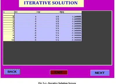
Manual calculations has been done as shown in Section 4.2 having optimum value as [-1, 3/2] and that were compared with the optimum solutions obtained with the help of software. It was found that they are nearly equal (see fig.3.a,b,c ) but hand calculations were time consuming. On the other hand software solved the problems in the fraction of seconds. It is user-friendly and requires a less computer knowledge or skill. The software is also well equipped with the theory behind the method. The user does not require searching for theory and this is one of the good things about the software which is developed for Newton’s method.
7. SOFTWARE SCREENS
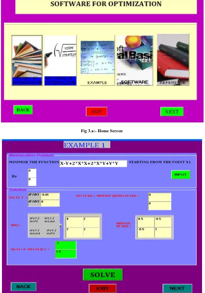
Fig 3.a:- Home Screen
[image:4.595.90.508.75.671.2]Fig 3.c:- Iterative Solution Screen
8. REFERENCES
[1] Optimization of Chemical Process, T.F. Edgar, D.M. Himmalblau, McGraw-Hill International Edition, Chemical series.
[2] Engineering Optimisation Theory And Practice, Third Edition, S.S. Rao
[3] Mathematics In Chemical Engineering, Bruce A. Finlayson, Lorentz T. Biegler, Ignacio E. Grossmann.
[4] Theory And Problems of Operation Research, Richard Bronson, Schaum’s Outline Series, Asian Students edition
[5] Operations Research An Introduction ,Fourth Edition, Hamdy A. Taha, Maxwell Macmillan Publishing Company, New York
[6] Higher Engineering Mathematics, 38th Edition, Dr. B. S.
Grewal, Khanna Publication
[7] Visual Basic-6 Programming Black Book, Steven Holzner, Dreamtech Press
[8] The Complete Reference Visual Basic 6, Noel Jerk, Tata McGraw Hill
[9] Mastering Visual Basic-6 Book
[10]Newton’s Method for Unconstrained Optimization ,Robert M. Freund February, 2004 , Massachusetts Institute of Technology.
[11] J. E. Dennis and R. B. Schnabel. Numerical methods for Unconstrained Nonlinear Equations.SIAM, Philadelphia, 1996.
[12]Iterative Methods for Optimization, C.T. Kelley, North Carolina State University, Raleigh, North Carolina