Monetary Policy and Inflation Dynamics
Roberts, John M
6 July 2006
John M. Roberts
Federal Reserve Board
Since the early 1980s, the U.S. economy has changed in some important ways: inflation now rises considerably less when unemployment is low, and the volatility of output and inflation have fallen sharply. This paper examines whether changes in monetary policy can account for these changes in the economy. The results suggest that changes in monetary policy can account for most or all of the change in the inflation-unemployment relationship. In addition, changes in policy can explain a large proportion of the reduction in the volatility of the output gap.
JEL Codes: E31, E32, E52, E61.
1. Introduction
In this paper, I assess the extent to which shifts in monetary pol-icy can account for an important change in the relationship between unemployment and inflation in the United States: it appears that, in a simple reduced-form Phillips curve relationship between changes in inflation and the unemployment rate, the estimated coefficient on unemployment has been considerably smaller since the early 1980s than it was earlier (Atkeson and Ohanian 2001; Staiger, Stock, and Watson 2001). In addition, I look at the ability of monetary policy to account for changes in the reduction in the volatility of output
∗I am grateful to Flint Brayton, David Lebow, Dave Stockton, and participants
at seminars at the Board of Governors, the Federal Reserve System’s macro-economics research committee, the NBER Monetary Economics program, and Harvard University for helpful discussions; to John Williams for providing his linearized version of the FRB/US model; and to Sarah Alves for able research assistance. The views expressed in this paper are those of the author and do not necessarily represent those of the Board of Governors of the Federal Reserve System or its staff.
and inflation that also dates from the early 1980s (McConnell and Perez-Quiros 2000).
The notion that monetary policy should affect inflation dynam-ics is an old one, dating at least to Friedman’s dictum that inflation is always a monetary phenomenon (1968). In his famous “Critique,” Lucas (1975) showed how changes in monetary policy could, in prin-ciple, affect inflation dynamics. However, Lucas considered only very stylized monetary policies. Here, I explore the effects of more realistic changes in policy on inflation dynamics.
I consider several ways in which U.S. monetary policy may
have changed. First, monetary policy may have become more
reac-tive to output and inflation fluctuations around the early 1980s (Clarida, Gal´ı, and Gertler 2000). In addition, monetary policy may have become more predictable, implying smaller shocks to a simple monetary-policy reaction function. Finally, Orphanides et al. (2000) argue that policymaker estimates of potential out-put may have become more accurate. Such improvements in esti-mates of potential output would constitute a change in monetary policy, as policy would be made on the basis of more accurate information.
I consider the effects of changes in policy on expectations formation, holding fixed the other behavioral relationships in the economy. Although other relationships are unchanged, changes in policy can nonetheless affect the reduced-form relationship between inflation and economic activity by reducing the signal content of economic slack for future inflation. For example, if monetary policy acts more aggressively to stabilize the economy, then any given deviation in output from potential will contain less of a sig-nal of future inflation. Similarly, a reduction in the persistence of potential output mismeasurement would mean that an increase in output resulting from a misestimate of potential output will not portend as much inflation because it is not expected to last as long.
near the extremes of the range of complexity among models currently employed in policy analysis.1
Ball, Mankiw, and Romer (1988) have argued that changes in monetary policy may lead to changes in the frequency of price adjust-ment and, thus, changes in the parameters of the price-adjustadjust-ment processes taken as structural here. In particular, they argue that the lower and more-stable inflation that has marked the post-1982 period is likely to lead to less-frequent price adjustment. The Ball-Mankiw-Romer conjecture could thus provide an alternative explanation for the reduction in the slope of the reduced-form Phillips curve. In a recent empirical study, however, Boivin and Giannoni (forthcoming) examined the sources of changes in the effects of monetary policy sur-prises on the economy. They found that the main source of changes in the effects of policy shocks was changes in the parameters of the policy reaction function rather than in the structural parameters of the economy, providing empirical support for the modeling strategy adopted here.
To summarize the results briefly, changes in monetary policy can account for most or all of the reduction in the slope of the reduced-form Phillips curve. Changes in policy can also account for a large portion of the reduction in the volatility of output gap, where the output gap is the percent difference between actual out-put and a measure of trend or potential outout-put. However, as in other recent work (Stock and Watson 2002; Ahmed, Levin, and Wilson 2004), changes in policy account for a smaller proportion of changes in output growth. The ability to explain the reduction in inflation volatility is mixed: in the small-scale model, it is pos-sible to explain all of the reduction in inflation volatility, whereas in FRB/US, the changes in policy predict only a small reduction in volatility. Finally, monetary policy’s ability to account for changes in the economy is enhanced when changes in monetary policy are broadened to include improvements in the measurement of potential GDP.
1
Table 1. The U.S. Economy’s Changing Volatility (Standard Deviations, Percentage Points)
Unem- Output Output GDP Core ployment Gap, Gap, Growtha
Inflationa
Rate FRB/US CBO
1984:Q1–2002:Q4 2.22 1.18 1.09 2.08 1.54
1960:Q1–1983:Q4 4.32 2.56 1.77 3.57 3.17
1960:Q1–1979:Q4 3.98 2.42 1.36 2.71 2.61
a
Quarterly percent change, annual rate.
2. The Changing Economy
2.1 Volatility of Output and Inflation
Table 1 presents standard deviations of the annualized rate of quar-terly GDP growth, core inflation (as measured by the annualized quarterly percent change in the price index for personal consumption expenditures other than food and energy), the civilian unemploy-ment rate, and two measures of the output gap. The table compares standard deviations from two early periods—1960–79 and 1960–83— with a more recent period, 1984–2002.
of the unemployment rate has fallen by 20 percent, but relative to the period ending in 1983, the decline is almost 40 percent.
The table also shows results for two measures of the output gap— one from the Federal Reserve’s FRB/US model and one from the
Congressional Budget Office (CBO).2 For the FRB/US gap
meas-ure, the 1984–2002 standard deviation is 23 percent less than in the 1960–79 period and 42 percent less than in the 1960–83 period. The declines in volatility are sharper for the CBO output gap, with a decline in standard deviation of 41 percent since the 1960–79 period and 51 percent since the 1960–83 period.
2.2 The Slope of the Reduced-Form Phillips Curve
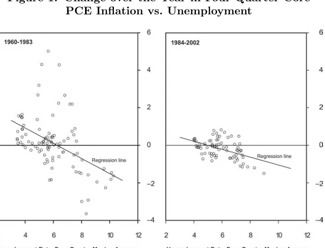
Figure 1 plots the over-the-year change in the four-quarter core PCE inflation rate against a four-quarter moving average of the unem-ployment rate. The panel on the left shows the scatter plot over the 1960–83 period; the panel on the right shows the scatter plot over the 1984–2002 period. Each panel includes a regression line; the slope coefficients are shown in the first column of table 2. The regression run is:
(pt−pt−4)−(pt−4−pt−8) =γ0+γ1(Σi=0,3 URt−i)/4, (1)
where (pt−pt−4) indicates the four-quarter percent change in core
PCE prices and UR is the civilian unemployment rate. As can be
seen in the table, the slope coefficient of this reduced-form Phillips curve falls by nearly half between either of the earlier periods and the post-1983 period. Atkeson and Ohanian (2001) have also noted a sharp drop in the slope of a similar reduced-form relationship, as have Staiger, Stock, and Watson (2001, figure 1.1).
Columns 2 and 3 of table 2 show the change in the slope co-efficient in equation (1), using the FRB/US and CBO output gaps,
2
Figure 1. Change over the Year in Four-Quarter Core PCE Inflation vs. Unemployment
Table 2. Evidence of a Shift in the Slope of the Reduced-Form Phillips Curve, Simple Model
(Equation 1)
Unemployment FRB/US CBO Rate Output Gap Output Gap
1984:Q1–2002:Q4 –.201 .092 .159
(.056) (.032) (.038)
1960:Q1–1983:Q4 –.389 .154 .207
(.085) (.050) (.043)
1960:Q1–1979:Q4 –.378 .130 .180
(.155) (.095) (.080)
[image:7.432.54.381.406.559.2]Table 3. Evidence of a Shift in the Slope of the Reduced-Form Phillips Curve, More Complex Model
(Equation 2)
Unemployment FRB/US CBO Rate Output Gap Output Gap
Slope Coefficient (γ1)
1984:Q1–2002:Q4 −.098 (.069) .051 (.036) .091 (.048) 1961:Q1–1983:Q4 −.154 (.052) .066 (.026) .084 (.028) 1961:Q1–1979:Q4 −.157 (.075) .056 (.038) .076 (.038)
Coefficient on First Inflation Lag (γ2)
1984:Q1–2002:Q4 .29 (.12) .29 (.12) .28 (.12) 1961:Q1–1983:Q4 1.02 (.10) 1.05 (.11) 1.02 (.10) 1961:Q1–1979:Q4 1.01 (.11) 1.04 (.12) 1.02 (.10)
respectively, in lieu of the unemployment rate. Results using the output gap provide a useful robustness check. In addition, the sim-ple three-equation model used below includes the output gap rather than the unemployment rate. The reduction in the Phillips-curve slope is smaller using the output gap: for the FRB/US output gap, the reduction is between 30 percent and 40 percent, depending on the reference period, whereas for the CBO output gap, the reduction is only 12 percent to 23 percent. (As might be expected given typi-cal Okun’s law relationships, the coefficients on the output gap are about half the size of the coefficients in the corresponding equations using the unemployment rate—and, of course, they have the opposite sign.)
In table 3, I look at an alternative specification of the reduced-form Phillips curve, in which the quarterly change in inflation is regressed on three lags of itself and the level of the unemployment rate:
∆pt=γ0+γ1URt+γ2∆pt−1+γ3∆pt−2
where ∆pt indicates the (annualized) one-quarter percent change
in the core PCE price index. As in equation (1), the coefficients on lagged inflation are constrained to sum to one. I discuss the evidence for this restriction in section 2.3. For the unemployment rate, the results are qualitatively similar to those in table 2, although the mag-nitude of the reduction in the slope is a bit less, as the coefficient falls by 35 percent to 40 percent. In this regression, there is also a notable drop-off in the statistical significance of the slope coefficient, with thet-ratio falling to 1.4 in the post-1983 sample, from levels of around 2 or 3 in the earlier samples.
For the estimates with the output gap in columns 2 and 3, the slope coefficients now change little between the early and late samples—indeed, for the CBO output gap, the coefficient even rises. However, in equation (2), the slope coefficient no longer summa-rizes the effect of unemployment on inflation, because the pattern of the coefficients on lagged inflation also matters. As can be seen in the bottom three rows of the table, there was an important shift in these coefficients, with the coefficient on the first lag dropping from around 1 in the early samples to a bit less than 0.3 in the post-1983 sample. This change means that, in the later sample, an initial shock to unemployment will have a much smaller effect on inflation in the following quarter than was the case in the earlier period. If the impact of unemployment on inflation is adjusted for this change in lag pattern, then the estimates in table 3 suggest that there has been a sharp reduction of the impact of the output gap on inflation, of between 50 percent and 67 percent.3Because the slope coefficient in
the simple model of equation (1) provides a single summary statistic for the change in the inflation dynamics, I will focus on changes in this coefficient in my work below.4
3
In particular, I compute a “sacrifice ratio,” which is the loss in output or unemployment required to obtain a permanent reduction of 1 percentage point in inflation.
4
2.3 Has U.S. Inflation Stabilized?
In the preceding subsection, it was assumed that the sum of coef-ficients on lagged inflation in the reduced-form Phillips curves remained equal to one. Of course, it is possible to imagine that if a central bank had managed to stabilize the inflation rate, inflation would no longer have a unit root, and the sum of lagged coeffi-cients in the reduced-form Phillips curve would no longer equal one. Ball (2000) argues that, prior to World War I, inflation was roughly stable in the United States, and the sum of lagged coefficients in reduced-form Phillips curves was less than one; Gordon (1980) makes a similar point.
It is not yet clear if inflation stability is once again a reality for the United States. Figure 2 plots the sum of lagged inflation coefficients from a rolling regression of U.S. core PCE inflation on four lags of itself, using windows of ten, fifteen, and twenty years. With a twenty-year window, the sum of lagged coefficients remains near 0.9 at the end of the sample, about where it was twenty years earlier. With a fifteen-year window, the sum is more variable, but here, too, it ends the sample at a high level. Using a ten-year window, there is more evidence that the persistence of inflation has fallen, as the sum of lagged coefficients drops to around 0.5.
The inflation data in the bottom panel helps explain these results. Inflation has moved down over the post-1983 period: infla-tion as measured by core PCE prices averaged 4 percent from 1984 to 1987 but only 11/2 percent over the 1998–2002 period. In the most
recent ten-year period, inflation has moved in a relatively narrow range, consistent with the small coefficient sum estimated over this period.
3. Changing Monetary Policy
3.1 Changes in the Reaction Function
One way to characterize the implementation of monetary policy is with a “dynamic Taylor rule” of the form:
fft=ρfft−1+ (1−ρ){r∗+ (p
t−pt−4) +αxgapt
+β[(pt−pt−4)−π ∗
t]}+ǫt, (3)
whereff is the federal funds rate,r∗ is the equilibrium real interest
rate, (pt−pt−4) is the four-quarter inflation rate,xgap is the GDP
gap, and π∗ is the target inflation rate. A number of studies have
found that such a rule characterizes monetary policy after 1983 quite well. Among others, these studies include Clarida, Gal´ı, and Gertler (CGG, 2000) and English, Nelson, and Sack (ENS, 2003).
While the dynamic Taylor rule appears to be a good character-ization of policy over the past two decades, its performance prior to 1980 is less impressive. For example, CGG find, in a similar model, very small estimates of the inflation parameter β—indeed, their point estimates putβat less than zero over the 1960–79 period. In this case, real interest rates will fail to rise when inflation is above target, which, as CGG discuss, can lead to an unstable inflation rate. CGG emphasize the increase in the value of β as indicating an important shift in monetary policy in the early 1980s. They also provide evidence that policy has become more responsive to out-put fluctuations, reporting a large increase inα. Taylor (1999) and Stock and Watson (2002) also find a large increase in the coefficient on output in a similar monetary policy rule.
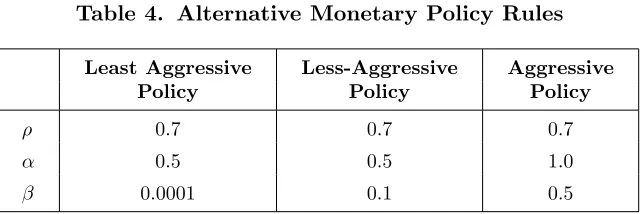
Table 4 summarizes the assumptions about monetary policy coef-ficients used in the simulations below. One set of parameters— labeled “aggressive”—is similar to the estimates of ENS for recent U.S. monetary policy. In the less-aggressive policy settings, the response to output is assumed to be half that in the aggressive set-ting, while the response to inflation is intended to be a minimal response that is consistent with stability.5
5
Table 4. Alternative Monetary Policy Rules
Least Aggressive Less-Aggressive Aggressive Policy Policy Policy
ρ 0.7 0.7 0.7
α 0.5 0.5 1.0
β 0.0001 0.1 0.5
[image:13.432.56.378.443.575.2]The reaction function in equation (3) includes an error term. One interpretation of such “shocks to monetary policy” is that they constitute changes to the objectives of monetary policy that are not fully captured by a simple econometric specification. Such an interpretation is perhaps most straightforward in a setting in which the long-run inflation objective of the central bank is not firmly established, as may have been the case for the United States in the pre-1980 period. In such a context, shocks to the reaction func-tion could correspond to changes in the inflafunc-tion target. Another interpretation—that the shocks represent errors in the estimation of the right-hand-side variables of the model—will be taken up shortly. Table 5 presents some evidence that the variability of the error term in the reaction function has fallen. The first column presents the unconditional standard deviation of the change in the quarterly average funds rate, which falls by between 40 percent and 55 percent, depending on the early reference period. The second column reports the standard error of the residuals from simple reduced-form models of the funds rate, in which the funds rate is regressed on four lags
Table 5. Volatility of the Federal Funds Rate (Standard Deviations, Percentage Points)
Residuals Change in from Reduced-Funds Rate Form Model
1984:Q1–2002:Q4 .56 .38
1960:Q1–1983:Q4 1.27 1.16
of itself, the current value and four lags of the FRB/US output gap, and the current value and four lags of quarterly core PCE inflation. This residual is considerably less variable in the post-1983 period, with the standard deviation falling by between 45 percent and 67 percent. In the simulations in sections 5 and 6, I will consider a reduction in the standard deviation of the shock to a monetary-policy reaction function like equation (3) of a bit more than half, from 1.0 to 0.47.
3.2 Improvements in Output Gap Estimation
As noted in the introduction, Orphanides et al. (2000) have sug-gested a specific interpretation for the error term—namely, that it reflects measurement error in the output gap. In particular, suppose that the monetary authorities operate under the reaction function:
fft=ρfft−1+ (1−ρ){r∗+ (pt−pt−4)
+α(xgapt+noiset) +β[(pt−pt−4)−π ∗
t]}, (4)
where,
noiset=φnoiset−1+ǫt. (5)
Here,noise has the interpretation of measurement error in the out-put gap. Orphanides et al. (2000) estimate the time-series process for ex post errors in the output gap by comparing real-time esti-mates of the output gap with the best available estiesti-mates at the end of their sample. They find that there was an important shift in the time-series properties of the measurement error in the output gap. In particular, for the period 1980–94, the serial correlation of output gap mismeasurement is 0.84, considerably smaller than the 0.96 serial correlation they find when they extend their sample back to 1966.6
6
The later period examined by Orphanides et al.—1980–1994—is earlier than the post-1983 period that has been characterized by reduced volatility and reduced responsiveness of inflation to the unemployment rate. It would thus be of interest to have an esti-mate of such errors for a more-recent period. The paper by English, Nelson, and Sack (2003) suggests an indirect method of obtaining such an estimate. They estimate a monetary-policy reaction func-tion similar to equafunc-tion (3), but with a serially correlated error term. When estimated using current-vintage data, such a model can be given an interpretation in terms of the reaction function with noisy output gap measurement in equations (4) and (5). This can be seen by rewriting equation (4) as
fft=ρfft−1+ (1−ρ){r∗+ (p
t−pt−4)
+αxgapt+β[(pt−pt−4)−πt∗]}+ut, (6)
where ut ≡ α(1−ρ) noiset, and is thus an AR(1) error process
because, as noted in equation (5), noiset is an AR(1) process.
The results of ENS suggest that the noise process had a root of 0.7 over the 1987–2001 period. Estimates of a model similar to theirs suggest that the standard deviation of the shock to the noise process was 1.2 percentage points—about the same as Orphanides et al. (2000) found for both their overall and post-1979 samples.7
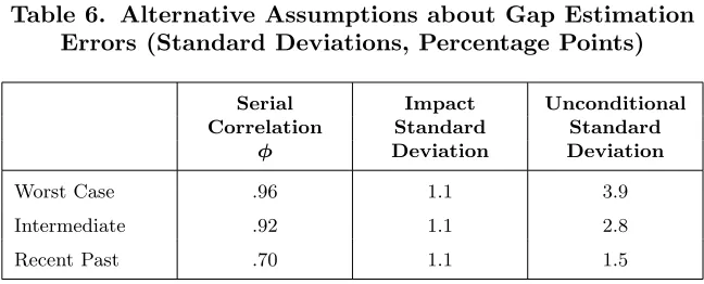
The preceding discussion suggests two extreme noise processes— the “worst-case” process identified by Orphanides et al. (2000), with a serial correlation parameter of 0.96, and the process implicit in the serial correlation process of the error term from a reaction function estimated with recent data, where φ= 0.70. I will also consider an intermediate case, with φ= 0.92, which can be thought of as a less-extreme version of the Orphanides et al. worst case. Because there is little evidence for a shift in the standard deviation of the shock to the noise process, I assume the same value for all three processes, 1.10. These assumptions are summarized in table 6.
7
Table 6. Alternative Assumptions about Gap Estimation Errors (Standard Deviations, Percentage Points)
Serial Impact Unconditional
Correlation Standard Standard
φ Deviation Deviation
Worst Case .96 1.1 3.9
Intermediate .92 1.1 2.8
Recent Past .70 1.1 1.5
3.3 Specification of the Inflation Target
As discussed in section 2.3, movements in inflation appear to have remained persistent in the 1983–2002 period. One reason for such persistence may be that the implicit inflation objective varied over this period. A specification that allows for inflation objectives to drift in response to actual events is
π∗
t =µπt∗−1+ (1−µ)∆pt, (7)
where, as before, ∆pt represents annualized inflation. In
equa-tion (7), a fixed inflaequa-tion target can be specified by setting µ = 1. Ifµ <1, however, then the inflation target will be affected by past inflation experience, and inflation will possess a unit root. In most of the simulations that follow, I assumeµ= 0.9. In simulations of the FRB/US model, this value ofµallows the model to capture the his-torical relationship between economic slack and persistent changes in inflation. The results are not greatly affected by small changes in this parameter.
4. Models
the three-equation model is that it can be thought of as including the minimal number of variables needed to model the monetary pol-icy process: the monetary-polpol-icy reaction function is combined with equations for its independent variables—inflation and the output gap. In addition, the model’s small size makes it straightforward to vary model parameters. The model is described more fully shortly.
The other model I use is the Federal Reserve’s large-scale FRB/US model. FRB/US is described in detail in Brayton et al. (1997) and Reifschneider, Tetlow, and Williams (1999). Among the key features of the FRB/US model are the following: the underly-ing structure is optimization based, decisions of agents depend on explicit expectations of future variables, and the structural parame-ters of the model are estimated. More-specific features of the model are discussed at the end of this section.
In both the three-equation model and FRB/US, economic agents are assumed to be at least somewhat forward looking, and they form model-consistent expectations of future outcomes. As a consequence, their expectations will be functions of the monetary policy rule in the model. In this way, these models are—at least to some extent— robust to the Lucas critique, which argues that agents’ expectations should change when the policy environment changes.
In addition to the monetary-policy reaction function described in section 3, the three-equation model also includes a New Keynesian Phillips curve and a simple “IS curve” that relates the current out-put gap to its lagged level and to the real short-term interest rate. The New Keynesian Phillips curve is
∆pt=Et∆pt+1+κxgapt+ηt, (8)
where ηt is an error term representing shocks to inflation. The
microeconomic underpinnings of such a model are discussed in vari-ous places—see, for example, Roberts (1995). Because equation (8) can be thought of as having an explicit structural interpretation, it will be referred to as the “structural Phillips curve,” in contrast to “reduced-form Phillips curves” such as equations (1) and (2).
Some recent work has focused on the possibility that inflation expectations are less than perfectly rational (Mankiw and Reis 2002). One way of specifying inflation expectations that are less than perfectly rational is
Et∆pt+1=ωMt∆pt+1+ (1−ω)∆pt−1, (9)
where the operatorM indicates rational or “mathematical” expec-tations. An interpretation of this specification is that only a frac-tion ω of agents use rational expectations, while the remainder use last period’s inflation rate as a simple rule of thumb for forecasting inflation. Substituting equation (9) into equation (8) yields
∆pt=ωMt∆pt+1+ (1−ω)∆pt−1+κ xgapt+ηt. (10)
Fuhrer and Moore (1995) and Christiano, Eichenbaum, and Evans (CEE, 2005) provide alternative microeconomic interpretations of equation (10). Fuhrer and Moore assume that agents are concerned with relative real wages. CEE argue that in some periods, agents fully reoptimize their inflation expectations, whereas in others, they simply move their wage or price along with last period’s aggregate wage or price inflation. In their model, wages and prices are reset each period and thus are only sticky for a very brief period. The only question is how much information is used in changing those wages and prices.
The theoretical models of both Fuhrer and Moore and CEE sug-gest thatω =1/2. The results of Boivin and Giannoni (forthcoming)
provide empirical support for ω = 1/
2. I will therefore assume ω is
about 1/2 in the simulations below.8 I discuss other aspects of the
calibration choice in section 6. The IS curve is
xgapt=θ1xgapt−1+ (1−θ1)Et xgapt+1−θ2(rt−2−r∗) +νt, (11)
8
To be precise, I assume ω = 0.475. I choose a value slightly less than 1/ 2
where r is the real federal funds rate and νt is a random shock
to aggregate demand. As in equations (3) and (4), r∗ is the
equi-librium real federal funds rate, which is assumed to be constant. One way to interpret the equation’s error term, νt, however, is as
a variation in r∗. Rotemberg and Woodford (1997) discuss how an
IS curve with θ1 = 0 can be derived from household optimizing
behavior. Amato and Laubach (2004) show how habit persistence can lead to a specification with lagged as well as future output. These papers also show how the equilibrium real interest rate, r∗, is related to the underlying preference parameters of
house-holds. The lagged effect of interest rates on output can be jus-tified by planning lags; Rotemberg and Woodford (1997) assume a similar lag. Again, details of the calibration are provided in section 6.
Stock and Watson (2002) also examine the effects of changes in monetary policy using a small macroeconomic model. Their model also has a reduced-form output equation, a model of inflation with explicitly forward-looking elements, and a monetary-policy reaction function; in addition, they include an equation for commodity prices. While Stock and Watson’s model includes several explicitly cali-brated parameters, it also includes a number of lag variables for which parameters are not reported, making a close comparison of the models difficult.
the stochastic simulations of the FRB/US model include technology shocks.9
5. Impulse Responses
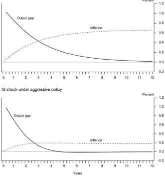
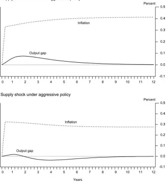
This section examines how the output and inflation effects of shocks to the model economy change under different monetary policies. Figure 3 shows the effects of a shock to the IS curve on output and inflation using the three-equation model discussed in the previ-ous section. The top panel shows the effects of the shock under the least aggressive monetary policy, while the bottom panel shows the effects under the aggressive policy. In both panels, the shock initially raises output and inflation. Because the inflation target is affected by past inflation, there is a permanent increase in inflation in both panels. However, under the aggressive policy in the bottom panel, output returns more rapidly to its preshock value, and the long-run increase in inflation is much smaller. Moreover, one to two years after the initial shock, the increase in inflation is notably smaller relative to output, suggesting a smaller reduced-form relationship between these variables under the aggressive policy.
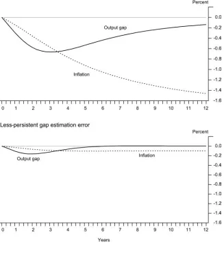
Figure 4 looks at the effects of a reduction in the persistence of output gap estimation errors, holding fixed the responsiveness of monetary policy at the aggressive level. The top panel considers the worst-case estimate for error persistence (φ= 0.96), while the bot-tom panel shows the recent-past case (φ = 0.7). As can be seen, an initial 1-percentage-point estimation error has much-larger and more-persistent effects on output and inflation in the top panel than in the bottom panel. Moreover, the impact of the shock on inflation over the first couple of years is much larger relative to the impact on inflation in the top panel, again suggesting a larger reduced-form slope.10
9
Footnote 2 contains additional information about the supply side of the FRB/US model.
10
Figure 3. Implications of a More-Aggressive Monetary Policy for the Effects of an IS Shock
Three-Equation Model
Figure 4. Effects of an Output Gap Estimation Error Three-Equation Model
Figure 5. Implications of a More-Aggressive Monetary Policy for the Effects of a Supply Shock
Three-Equation Model
bottom panel, however, real interest rates eventually rise relative to baseline, so there is a period of negative output gaps. The eventual increase in inflation is thus smaller than under the least aggressive policy, although, once again, because the inflation target is allowed to be endogenous, inflation is permanently higher.
Of course, the simulations in figures 3 through 5 show only the effects of individual shocks. By contrast, the empirical reduced-form Phillips-curve coefficients such as those discussed in section 2 reflect the effects of all shocks. A convenient way to consider the joint effect of a number of shocks on the reduced-form coefficients is stochastic simulation, the subject of the next section.
6. Stochastic Simulations
6.1 Results with the Three-Equation Model
In this subsection, I use the three-equation model to assess how changes in monetary policy affect volatility and the relationship between inflation and unemployment.
To calibrate the IS curve of the model, I first chose a weight on future output, θ1, of 1/2, similar to the degree of forward
look-ing assumed in the structural Phillips curve discussed above. I then chose the IS-curve slope, θ2, so as to match the effect of an
iden-tified monetary policy shock on output in a VAR estimated over the 1960–2002 period, which implied θ2 = 0.1. I chose the slope of
the structural Phillips curve and the standard errors of the shocks to the IS and structural Phillips curves so as to approximate the volatility of output, the volatility of inflation, and the slope of the simple reduced-form Phillips curve. This exercise resulted in stan-dard deviations of the IS and Phillips-curve shocks of 0.55 percent-age point and 0.17 percentpercent-age point, respectively, and a structural Phillips-curve slope of 0.005. Note that the model has been cal-ibrated so that the volatility of the residuals is representative of the low-volatility period for the U.S. economy. The IS and Phillips-curve parameter estimates are in broad agreement with empirical estimates of New Keynesian models, such as Boivin and Giannoni (forthcoming).
generate simulated data by taking random draws from the distri-bution of the model residuals. For each draw, a time series of 160 quarters is created. To reduce the influence of starting values, the first eighty quarters are discarded, and sample statistics are com-puted using the last eighty quarters. The shocks are drawn from a normal distribution.
The standard deviation of output growth, the output gap, and inflation are calculated for each draw, and the summary statistics are averaged over the draws. Similarly, the slope of the reduced-form Phillips curve is estimated for each draw. I present the slope coef-ficients from two models. One is the simple reduced-form Phillips curve of equation (1), modified to use the output gap rather than the unemployment rate:
(pt−pt−4)−(pt−4−pt−8) =γ0+γ1 (Σi=0,3xgapt−i)/4. (12)
Presenting results for this simple model has the advantage that the results are directly comparable to the simple relations illustrated in figure 1; also, the results focus attention (and econometric power) on the slope coefficient. I also consider the slightly more elaborate reduced-form Phillips curve:
∆pt=γ0+γ1xgapt+γ2∆pt−1
+γ3∆pt−2+γ4∆pt−3+γ5∆pt−4. (13)
Equation (13) is similar to equation (2) except that, here, the sum of the lagged inflation coefficients is not constrained to sum to one. Estimates of this equation can thus allow for the possibility that the changes in policy under consideration may have reduced the sum of lag coefficients.11
In table 7, I consider the effects of changes in the coefficients of the reaction function and changes in the volatility of a simple i.i.d. error term added to the reaction function. These changes in policy are similar to those that Stock and Watson (2002) have considered. I later turn to the possibility that the serial correlation of errors in the measurement of the output gap may have fallen. Initially, to
11
Table 7. The Effects of Changes in Monetary Policy on Volatility and the Slope of the Reduced-Form
Phillips Curve: Three-Equation Model
(1) (2) (3) (4)
Inflation Target: Evolving Evolving Evolving Fixed M-policy Shock: S.D. = 1.0 S.D. = 1.0 S.D. = 0.47 S.D. = 0.47
αandβ: 0.5 and 0.0001 1.0 and 0.5 1.0 and 0.5 1.0 and 0.5
Volatility:
S.D. (Gap) 2.32 1.82 1.79 1.84 S.D. (Inflation) 2.36 1.20 1.19 1.02
Phillips Curves:
Simple; Slope .213 .139 .139 .146 (.073) (.084) (.086) (.085) With Lags; Slope .062 .041 .041 .040
(.024) (.026) (.026) (.026) Sum Lag Coefs. .98 .94 .94 .93
(.03) (.06) (.06) (.06)
Inflation, .97 .94 .94 .92
Largest Root (.03) (.05) (.05) (.05)
Notes:Numbers in parentheses are standard errors.
“Sum lag coefs.” indicates the sum of the coefficients on lagged inflation.
Based on stochastic simulations with 5,000 draws.
isolate the effects of these changes in policy from the possibility that target inflation has become better anchored, I assume that target inflation is updated using equation (7) with a parameterµ= 0.9.
while the reduction in inflation volatility is in line with that seen historically.12
The slope of the simple reduced-form Phillips curve falls by about one-third, in line with historical reductions in the Phillips-curve slope as measured with the output gap, although somewhat short of the reductions in the coefficient on the unemployment rate. Also, the t-statistic on the slope of the simple Phillips curve falls from 2.9 to 1.6, suggesting that these changes in monetary policy may also have affected the apparent statistical robustness of the simple Phillips-curve relationship. The more-elaborate Phillips curve shows a similar reduction in slope, while the sum of coefficients on lagged inflation remains high.13
Column 3 introduces an additional change in monetary policy, a reduction in the volatility of the shock to policy. In this model, this additional change has very little effect on the results: the volatility of the output gap and inflation fall somewhat more, but the estimated Phillips-curve slopes are very similar to those in column 2.
Column 4 looks at the implications of the switch to a fixed infla-tion target, under the assumpinfla-tion of an aggressive monetary policy and small shocks to the reaction function, as in column 3. This shift in policy has only small effects on the results: the volatility of the output gap actually rises a bit, while that of inflation falls by about 15 percent. The slope of the reduced-form Phillips curve rises a bit. Perhaps surprisingly, the persistence of inflation falls only slightly, and inflation remains highly persistent. In section 7, I return to the question of how the behavior of the economy might change if the central bank were to adopt a strict inflation target.
12
It is worth noting that this improvement in both output and inflation volatil-ity is not at variance with Taylor’s (1979) well-known volatilvolatil-ity trade-off. Taylor’s trade-off described the choice among alternative optimal policies, whereas the policy changes I am examining here represent a shift from policies that are well outside the optimality frontier toward policies that are closer to that frontier.
13
Table 8. The Effects of Changes in the Persistence of Potential Output Errors on Volatility and the
Slope of the Reduced-Form Phillips Curve: Three-Equation Model
(1) (2) (3) (4) (5)
Error Persistence: 0.96 0.96 0.92 0.7 0.7 Inflation Target: Evolving Fixed Evolving Evolving Fixed
αandβ: 0.5 & 0.1 1.0 & 0.5 0.5 & 0.1 1.0 & 0.5 1.0 & 0.5
Volatility:
S.D. (Gap) 3.51 2.64 2.68 1.82 1.88 S.D. (Inflation) 6.71 2.37 3.31 1.22 1.05
Phillips Curves:
Simple; Slope .289 .221 .239 .145 .150 (.066) (.068) (.070) (.085) (.082) With Lags: Slope .069 .059 .064 .043 .043
(.024) (.022) (.023) (.026) (.026) Sum Lag Coefs. .99 .97 .98 .94 .93
(.02) (.03) (.03) (.06) (.06)
Inflation, .99 .97 .98 .94 .93 Largest Root (.02) (.03) (.03) (.05) (.05)
Notes:Numbers in parentheses are standard errors.
“Sum lag coefs.” indicates the sum of the coefficients on lagged inflation.
[image:28.432.53.378.130.425.2]Based on stochastic simulations with 5,000 draws.
reaction-function parameters along with a fixed inflation target.14
With this policy, the volatility of the output gap is about in line with historical values for the 1960–79 period, and inflation is much closer to the historical range. The slope of the simple reduced-form Phillips curve is just above the historical range. Inflation is highly persistent, with a root of 0.97. These results are consistent with the argument made in Orphanides (2001) that poor estimation of poten-tial output, rather than weak response of monetary policy to output and inflation, was responsible for volatile and persistent inflation in the pre-1984 period.
In column 3, I consider an alternative in which the monetary policy reaction remains weak, but output gap errors are somewhat less persistent than in columns 1 and 2. This adjustment cuts the standard deviation of inflation by more than half, bringing it closer to the range that was seen historically. Both columns 2 and 3 provide plausible candidate characterizations of the high-volatility period.
Column 4 considers the implications of a reduction in the persis-tence of the shock to the reaction function, so thatφ= 0.7, under the assumption of an aggressive monetary policy. As can be seen by com-paring column 4 with column 2, reducing the persistence of the shock to the reaction function while holding the parameters of the reac-tion funcreac-tion fixed has important effects on the volatility of output and the slope of the Phillips curve. The standard deviation of the output gap falls by 30 percent, and the volatility of inflation falls by almost half. The slope of the simple Phillips curve falls by about one-third. As in table 7, there is a marked reduction in the statisti-cal significance of the Phillips-curve slope, as the t-ratio falls from more than 3 to just 1.7. Inflation remains highly persistent, with an autoregressive root of 0.94.
Comparing column 4 with column 3 gives an alternative view of the change in monetary policy—namely, that it represented a com-bination of more-aggressive policy and better estimation of poten-tial output. The story on output volatility is about the same as for column 2. The reduction in the slope of the simple reduced-form Phillips curve is greater in this case, at around one-half.
14
The final column of table 8 adds the assumption of a fixed infla-tion target. The volatility of inflainfla-tion falls somewhat further, while that of the output gap rises a bit. Estimates of the slope of the Phillips curve are little changed. As in table 7, the adoption of a fixed inflation target has surprisingly little effect on the persistence of inflation in this model.
6.2 Results with FRB/US
In this section, I work with the Federal Reserve’s FRB/US model of the U.S. economy. In the simulations, I solve a linearized version of the FRB/US model under model-consistent expectations. The draws for the stochastic simulations are taken from a multivariate normal distribution using the variance-covariance matrix of residuals from the FRB/US model estimated over the 1983–2001 period. Hence, the volatility of the residuals is representative of the low-volatility period for the U.S. economy. Because the FRB/US model includes the unemployment rate, these reduced-form Phillips-curve results are based on this variable, as in equations (1) and (2).
Columns 1, 2, and 3 of table 9 consider the effects of first increas-ing the parameters of the reaction function and then reducincreas-ing the volatility of the (not serially correlated) shock to the reaction func-tion. As in table 7, it is primarily the change in the reaction-function parameters that affects the volatility of output; there is only a small further reduction from reducing the volatility of the reaction-function shock. Between column 1 and column 3, the standard
devi-ation of the GDP gap falls by about 30 percent, somewhat more
than with the three-equation model. However, the standard devia-tion of GDP growth falls by only about 10 percent. The reduction in the volatility of the output gap is in the range of the historical decline between the 1960–79 and 1983–2002 periods. But the reduc-tion in GDP growth volatility is considerably smaller than what actually occurred, a finding similar to that of Stock and Watson (2002).
Table 9. The Effects of Changes in Monetary Policy on Volatility and the Slope of the Reduced-Form
Phillips Curve: FRB/US
(1) (2) (3) (4)
Inflation Target: Evolving Evolving Evolving Fixed M-policy Shock: S.D. = 1.0 S.D. = 1.0 S.D. = .47 S.D. = .47
αandβ: 0.5 and 0.0001 1.0 and 0.5 1.0 and 0.5 1.0 and 0.5
Volatility:
S.D. (Gap) 2.4 1.8 1.7 1.9
S.D. (GDP Growth) 3.5 3.2 3.2 3.1 S.D. (Inflation) 2.8 3.2 3.2 1.6
Phillips Curves:
Simple; Slope −.186 −.176 −.129 −.081
(.279) (.394) (.409) (.278) With Lags; Slope −.130 −.074 −.054 −.081
(.179) (.198) (.205) (.181) Sum Lag Coefs. .84 .89 .89 .71
(.12) (.10) (.10) (.20)
Inflation, .89 .92 .92 .77
Largest Root (.07) (.07) (.07) (.11)
Notes:Numbers in parentheses are standard errors.
“Sum lag coefs.” indicates the sum of the coefficients on lagged inflation.
Based on stochastic simulations with 2,000 draws.
With the reduction in the volatility of the monetary policy shock in column 3, the slope of the simple Phillips curve relative to column 1 is now about one-third smaller. The slope of the more-elaborate Phillips curve also declines further, and the total reduction is now almost 60 percent. As in the three-equation model, these changes in monetary policy can account for most or all of the reduction in the slope of the reduced-form Phillips curve.
Table 10. The Effects of Changes in the Persistence of Potential Output Errors on Volatility and the Slope of the Reduced-Form Phillips Curve:
FRB/US
(1) (2) (3) (4) (5)
Error Persistence: 0.96 0.96 0.90 0.70 0.70 Inflation Target: Evolving Fixed Evolving Evolving Fixed
αandβ: 0.5 & 0.1 1.0 & 0.5 0.5 & 0.1 1.0 & 0.5 1.0 & 0.5
Volatility:
S.D. (Gap) 6.1 3.4 3.5 1.8 1.9 S.D. (GDP Growth) 5.8 4.0 4.1 3.2 3.1 S.D. (Inflation) 6.3 3.6 3.7 3.3 1.7
Phillips Curves:
Simple; Slope −.47 −.50 −.33 −.17 −.102
(.16) (.20) (.22) (.41) (.26) With Lags; Slope −.37 −.35 −.22 −.070 −.093
(.18) (.16) (.17) (.21) (.18) Sum Lag Coefs. .83 .84 .84 .89 .71
(.09) (.09) (.11) (.11) (.20)
Inflation, .94 .92 .92 .92 .77 Largest Root (.04) (.06) (.05) (.07) (.11)
Notes:Numbers in parentheses are standard errors.
“Sum lag coefs.” indicates the sum of the coefficients on lagged inflation.
Based on stochastic simulations with 2,000 draws.
and small shocks to the reaction function, as in column 3. In con-trast to the three-equation model, there is now a large reduction in inflation persistence with the switch to a fixed inflation target, a result perhaps more in line with prior expectations.
inflation (column 1) leads to volatilities of output and inflation that are far greater than was the case historically. For inflation, this result is similar to that in table 8; for the output gap, the excess volatility is much greater. Columns 2 and 3 repeat the two solutions to this excess volatility used with the three-equation model: (i) assuming a more-aggressive policy and (ii) assuming somewhat smaller per-sistence of estimation errors. Both solutions reduce the volatility of output and inflation, and both lead to plausible characterizations of the earlier period.
Column 4 considers the implications of a reduction in the persis-tence of the shock to the reaction function, so that φ= 0.7, under the assumption of an aggressive monetary policy. As can be seen by comparing column 4 with column 2, reducing the persistence of the shock to the reaction function while holding the parameters of the reaction function fixed has large effects on the volatility of the output gap and the slope of the Phillips curve. The standard devi-ation of the output gap falls by almost half, at the high end of the range of the historical decline. However, the reduction in the stan-dard deviation of outputgrowth is only about 20 percent. The slope of the simple Phillips curve falls by two-thirds—even more than the declines that have been seen historically. Inflation remains highly persistent, with an autoregressive root of 0.92. The comparison of column 4 with column 3 yields similar results for output volatility. The reduction in the slope of the simple reduced-form Phillips curve is less sharp in this case, but it is still around 40 percent.
While the FRB/US model predicts reductions in output gap volatility and the slope of the Phillips curve that are consistent with historical changes, it does not suggest that monetary policy had much to do with the reduction in inflation volatility. Looking across tables 9 and 10, changes in policy lead to reductions of the standard deviation of inflation of at most 10 percent, well short of the historical reductions.
7. How Might the Economy Behave under a Fixed Inflation Target?
As figure 2 suggested, the evidence for a drop in inflation persis-tence is, thus far, inconclusive. However, estimates limited to the past decade are suggestive that inflation may have become more sta-ble. In this section, I use the three-equation model to consider how the behavior of the economy may change in a regime of inflation stability.
Expectations formation is central to the question of how infla-tion dynamics are likely to change in a regime of inflainfla-tion stability. In the simulations considered so far, equation (9) has been used as the model of expectations formation. In equation (9), “nonoptimiz-ing” agents rely on past inflation as an indicator of future inflation. Similarly, under CEE’s interpretation of the model, agents find it useful to use lagged inflation to index prices in periods when they do not reoptimize. It is most useful to use lagged inflation as a predic-tor of future inflation when inflation is highly persistent; if inflation were not persistent, lagged inflation would not be a good indicator of future inflation. It is reasonable to assume, therefore, that if inflation were to be stabilized, agents would change their inflation forecast-ing rules. Here, I consider one characterization of how agents might change the way they set expectations as inflation dynamics change. In particular, I consider the following generalization of equation (9):
Et∆pt+1=ωMt∆pt+1+ (1−ω)λ∆pt−1, (14)
where the parameterλis chosen so as to give the best “univariate” forecast of inflation. (For simplicity, the implicit inflation target is assumed to be zero.) Thus, in equation (9),λ= 1 was the best uni-variate forecast under the assumption—which has heretofore been close to accurate—that inflation had a unit root.
however, further reduces the persistence of inflation. Following this process to its logical conclusion suggests that a “fixed point” for uni-variate expectations formation is approximately zero autocorrelation (actually, the fixed point is λ= 0.02).
According to this model, then, the long-run consequences of a policy of a fixed inflation target is inflation that is not only station-ary but actually uncorrelated. Of course, this evolution is based on a particular assumption about expectations formation. But there is some historical precedent for such an outcome. Ball (2000) argues that in the 1879–1914 period, when the United States was on the gold standard, the “best univariate forecast” for inflation was zero: under the gold standard, inflation was not expected to persist. Ball (2000) and Gordon (1980) argue that allowing perceived inflation dynamics to change with the policy regime can go a long way to allowing the expectations-augmented Phillips curve—which works well in the second half of the twentieth century—to account for the properties of inflation under the gold standard.
If a central bank were to adopt a fixed inflation target, how quickly might a transition to stable inflation take place? Based on simulations with the baseline three-equation model, it could take a while for agents to catch on. In table 7, for example, inflation is predicted to have an autoregressive root of 0.92 even under a fixed inflation target. In the twenty-year sample underlying these simula-tions, thet-ratio of the hypothesis that this coefficient is still one is only 1.6, well short of Dickey-Fuller critical values. So even if agents with univariate expectations were good time-series econometricians, they may see little need to change the way they form their expec-tations. FRB/US, however, is more sanguine: switching to a fixed inflation target leads to a large reduction in the persistence of infla-tion, and the largest root of inflation falls to 0.77 (table 9, column 4, and table 10, column 5). If this were the case, the transition to stable inflation could occur more rapidly.
8. Conclusions
large declines in the slope of the reduced-form relationship between the change in inflation and the unemployment rate, holding fixed the structural parameters underlying inflation behavior. This result holds both in the large-scale FRB/US model and in a small New Keynesian-style model.
These changes in policy also have implications for the volatility of output and inflation—which also changed in the early 1980s. The results for inflation volatility were mixed: in the small model, changes in monetary policy can account for most or all of the reduction in the standard deviation of inflation. By contrast, in FRB/US, these monetary policy changes predict only a small reduction in inflation volatility.
The paper considered two alternative views of the change in monetary policy. One view is that the responsiveness of monetary policy to output and inflation increased, along the lines suggested by Clarida, Gal´ı, and Gertler (2000). I also considered the implica-tions of an alternative view of the change in the monetary policy process suggested by Orphanides et al. (2000)—that policymakers may have improved their methods for estimating potential GDP. This alternative view strengthens the ability of monetary policy changes to explain changes in the economy, implying greater reduc-tions in volatility and in the slope of the reduced-form Phillips curve.
through these possibilities would be an interesting topic for future research.
References
Ahmed, S., A. Levin, and B. A. Wilson. 2004. “Recent U.S. Macro-economic Stability: Good Policies, Good Practices, or Good Luck?”Review of Economics and Statistics 86 (3): 824–32. Amato, J. D., and T. Laubach. 2004. “Implications of Habit
Forma-tion for Optimal Monetary Policy.” Journal of Monetary
Eco-nomics 51 (2): 305–25.
Atkeson, A., and L. H. Ohanian. 2001. “Are Phillips Curves Useful for Forecasting Inflation?”Federal Reserve Bank of Minneapolis Quarterly Review 25 (1): 2–11.
Ball, L. 2000. “Near-Rationality and Inflation in Two Monetary Regimes.” NBER Working Paper No. 7988 (October).
Ball, L., N. G. Mankiw, and D. Romer. 1988. “New Keynesian
Eco-nomics and the Output-Inflation Trade-Off.” Brookings Papers
on Economic Activity 1:1–82.
Blanchard, O., and J. Simon. 2001. “The Long and Large Decline in U.S. Output Volatility.”Brookings Papers on Economic Activity 1:135–64.
Boivin, J., and M. Giannoni. Forthcoming. “Has Monetary Policy Become More Effective?”Review of Economics and Statistics88. Brayton, F., E. Mauskopf, D. Reifschneider, P. Tinsley, and J. C. Williams. 1997. “The Role of Expectations in the FRB/US
Macroeconomic Model.” Federal Reserve Bulletin 83 (April):
227–24.
Christiano, L. J., M. Eichenbaum, and C. L. Evans. 2005. “Nomi-nal Rigidities and the Dynamic Effects of a Shock to Monetary Policy.”Journal of Political Economy 113 (1): 1–45.
Clarida, R., J. Gal´ı, and M. Gertler. 2000. “Monetary Policy Rules and Macroeconomic Stability: Evidence and Some Theory.” Quarterly Journal of Economics 115 (1): 147–80.
Congressional Budget Office. 2001. CBO’s Method for Estimating
Potential GDP, available at www.cbo.gov.
Friedman, M. 1968. “Inflation: Causes and Consequences.” In Dol-lars and Deficits: Living with America’s Economic Problems, 21–60. Englewood Cliffs, NJ: Prentice-Hall.
Fuhrer, J., and G. Moore. 1995. “Inflation Persistence.” Quarterly Journal of Economics 110 (1): 127–59.
Gordon, R. J. 1980. “A Consistent Characterization of a Near-Century of Price Behavior.” American Economic Review 70 (2): 243–49.
Levin, A. T., V. Wieland, and J. C. Williams. 1999. “Robustness of
Simple Monetary Rules under Model Uncertainty.” InMonetary
Policy Rules, ed. J. B. Taylor. Chicago: University of Chicago Press.
Lucas, R. E. 1975. “Econometric Policy Evaluation: A Critique.” Carnegie-Rochester Conference Series 1:19–46.
Mankiw, N. G., and R. Reis. 2002. “Sticky Information ver-sus Sticky Prices: A Proposal to Replace the New Keynesian Phillips Curve.” Quarterly Journal of Economics 117 (4): 1295– 1328.
McConnell, M. M., and G. Perez-Quiros. 2000. “Output Fluctua-tions in the United States: What Has Changed Since the Early
1980s?” American Economic Review 90 (5): 1464–76.
Orphanides, A. 2001. “Monetary Policy Rules Based on Real-Time
Data.” American Economic Review 91 (4): 964–85.
Orphanides, A., R. D. Porter, D. Reifschneider, R. Tetlow, and F. Finan. 2000. “Errors in the Measurement of the Output Gap and the Design of Monetary Policy.” Journal of Economics and Business 52 (1–2): 117–41.
Reifschneider, D., R. Tetlow, and J. C. Williams. 1999. “Aggregate Disturbances, Monetary Policy, and the Macroeconomy: The
FRB/US Perspective.” Federal Reserve Bulletin 85 (January):
1–19.
Roberts, J. M. 1995. “New Keynesian Economics and the Phillips Curve.” Journal of Money, Credit, and Banking 27:975–84. ———. 2004. “Monetary Policy and Inflation Dynamics.” Federal
Reserve Board Finance and Economic Discussion Series Paper
No. 2004-62 (October).
Rotemberg, J. J., and M. J. Woodford. 1997. “An Optimization-Based Econometric Framework for the Evaluation of
ed. B. S. Bernanke and J. J. Rotemberg, 297–345. Cambridge, MA: MIT Press.
Rudebusch, G. D. 2005. “Assessing the Lucas Critique in Monetary Policy Models.”Journal of Money, Credit, and Banking 37 (2): 245–72.
Staiger, D., J. H. Stock, and M. W. Watson. 2001. “Prices, Wages, and the U.S. NAIRU in the 1990s.” InThe Roaring Nineties: Can Full Employment Be Sustained? ed. A. B. Krueger and R. M. Solow, 3–60. New York: Russell Sage Foundation.
Stock, J. H., and M. W. Watson. 2002. “Has the Business Cycle
Changed and Why?” In NBER Macroeconomics Annual, ed.
M. Gertler and K. Rogoff, 159–218. Cambridge, MA: MIT Press. Taylor, J. B. 1979. “Estimation and Control of a Macroeconomic Model with Rational Expectations.”Econometrica 47 (5): 1267– 86.