Munich Personal RePEc Archive
Outlier Treatment and Robust
Approaches for Modeling Electricity
Spot Prices
Trueck, Stefan and Weron, Rafal and Wolff, Rodney
Hugo Steinhaus Center, Wroclaw University of Technology
August 2007
Online at
https://mpra.ub.uni-muenchen.de/4711/
Outlier Treatment and Robust Approaches for Modeling Electricity
Spot Prices
∗Tr¨uck, Stefan
Macquarie University, Department of Economics Sydney, 2109 NSW, Australia
E-mail: strueck@efs.mq.edu.au
Weron, Rafa l
Wroc law University of Technology, Hugo Steinhaus Center Wyb. Wyspia´nskiego 27, 50-370 Wroc law, Poland
E-mail: rafal.weron@pwr.wroc.pl
Wolff, Rodney
Queensland University of Technology, School of Economics and Finance GPO Box 2434, Brisbane QLD 4001, Australia
E-mail: r.wolff@qut.edu.au
Abstract. We investigate the effects of outlier treatment on the estimation of the seasonal component and stochastic models in electricity markets. Typically, electricity spot prices exhibit features like seasonality, mean-reverting behavior, extreme volatility and the occurrence of jumps and spikes. Hence, an important issue in the estimation of stochastic models for electricity spot prices is the estimation of a component to deal with trends and seasonality in the data. Unfortunately, in regression analysis, classical estimation routines like OLS are very sensitive to extreme observations and outliers. Improved robustness of the model can be achieved by (a) cleaning the data with some reasonable procedure for outlier rejection, and then (b) using classical estimation and testing procedures on the remainder of the data. We examine the effects on model estimation for different treatment of extreme observations in particular on determining the number of outliers and descriptive statistics of the remaining series after replacement of the outliers. Our findings point out the substantial impact the treatment of extreme observations may have on these issues.
Introduction
In the last two decades the power sectors worldwide have undergone a transition from monop-olistic, government controlled systems into deregulated, competitive markets (Bunn, 2004; Harris, 2006; Kaminski, 2004; Kirschen and Strbac, 2004; Weron, 2006). The amount of risk borne by mar-ket participants has increased substantially, partially due to the fact that electricity is a very unique commodity. Firstly, it cannot be stored economically and requires immediate delivery, while end-user demand shows high variability and strong weather and business cycle dependence. Secondly, effects like power plant outages or transmission grid (un)reliability add complexity and randomness. Con-sequently, electricity spot prices exhibit very high volatility and abrupt, short-lived and generally unanticipated extreme price changes known as spikes (or jumps). The latter are, perhaps, the most distinct feature of deregulated power markets, and will be investigated in this paper.
Apart from the aforementioned spikes, the two other most prominent characteristics of spot elec-tricity prices include seasonality (at the annual, weekly and daily time horizons) and mean-reversion. The first crucial step in defining a model for electricity price dynamics consists of finding an appropriate description of the seasonal pattern. There are different suggestions for dealing with this task: Bhanot
∗Paper presented at the 56th Session of the International Statistical Institute, Invited Paper Meeting IPM71 ‘Statistics
(2000), Knittel and Roberts (2005) and Lucia and Schwartz (2002) use piecewise constant functions; Cartea and Figueroa (2005), Pilipovic (1997) and Weron et al. (2004a) model the seasonal pattern by sinusoidal functions; while Stevenson (2001) and Weron (2006) utilize a wavelet decomposition.
A critical issue in estimation of the seasonal pattern is that it might be substantially affected by the price spikes. While it is clear that price spikes should be captured by an adequate stochastic model, like jump-diffusion (Clewlow and Strickland, 2000; Geman and Roncoroni, 2006; Weron, 2007) or a regime-switching model (Bierbrauer et al., 2004; De Jong, 2006; Huisman and Mahieu, 2003), the literature does not agree on whether these observations have to be included or excluded in the estimation of the seasonal pattern. Even worse: despite the fact that price spikes are among the most pronounced features of electricity markets and account for a large part of the total variation of changes in spot prices, there is no commonly accepted definition of a price spike (Weron, 2006). A variety of methods for identification has been suggested, however, so far there has been no thorough empirical study on the effects of alternative treatment of the price spikes on parameter estimates for the seasonal pattern or the stochastic component of the spot price. It is exactly our goal to examine the consequences of the treatment of such extreme events in the estimation procedures. To identify the spikes we will consider a variety of different approaches. After such ‘cleaning’ of the observed spot prices we will then compare the remaining seasonal patterns.
Price Spikes
The identification of spikes is a very important issue as it bears on the estimation of the de-terministic and stochastic components for models of electricity spot price dynamics. However, in the literature the definition of a spike so far has been a rather subjective matter. Obviously, price spikes are defined as prices that surpass a specified threshold for a brief period of time. But it is difficult to gain any consensus on what that threshold or time interval should be.
Some authors use fixed price thresholds to identify the spikes (Lapuerta and Moselle, 2001). Other references suggest the use of fixed log-price change thresholds, e.g., log-price increments or returns exceeding 30% (Bierbrauer et al., 2004), or variable price change thresholds, e.g., log-price increments or returns exceeding three standard deviations of all log-price changes (Cartea and Figueroa, 2005; Clewlow and Strickland, 2000; Weron et al., 2004b). Borovkova and Permana (2004) considered as jumps those price moves that were outside 90% prediction intervals, implied by the normal distribution with the mean and variance given by the 60-days moving average and 60-days moving variance of the price moves. Yet another approach was used by Geman and Roncoroni (2006) who filtered raw price data using different thresholds and selected the one leading to the best calibrated model in view of its ability to match the kurtosis of observed daily price variations. Finally, the use of wavelet decomposition to filter out the spikes has been suggested (Stevenson, 2001; Weron, 2006). Obviously, different definitions and techniques may lead to quite different results and identification of price spikes.
The Data
0 200 400 600 800 1000 1200 1400 1600 1800 2000 0
50 100 150 200 250 300 350
Time (days)
Spot Price
Figure 1: Spot prices of the EEX Phelix Base (day) index from January 1, 2001, to December 31, 2006, totaling 2191 observations.
particular day.
Our data comprise six years of Phelix base day prices from January 1, 2001, to December 31, 2006, totaling 2191 observations. The dynamics of the spot prices for the considered period are shown in Figure 1. Obviously, several spikes can be observed during the considered period. For example, spot prices peaked in December 2001 with a daily average of 240 EUR/MWh, in January 2003 with 163 EUR/MWh and in July and November 2006 with 301 and 162 EUR/MWh, respectively. In most cases the spikes lasted only for one or two days and prices fell back to their normal levels very quickly. There is also an obvious trend in the data such that the average price level at the end of the considered period was substantially higher than in the first two-three years.
Methods to Detect the Spikes
Probably the simplest technique to detect outliers is the use of fixed price thresholds. However, the choice of the levels themselves is non-trivial and rather arbitrary. For the present dataset, we chose to classify all prices beyond 75 EUR/MWh as extreme observations. Obviously other thresholds may be chosen depending on needs.
Nevertheless, the remaining question is how to replace the outliers. The chosen technique for replacement will also affect parameter estimates, e.g., of the seasonal pattern if the estimation is con-ducted using the new series. Some authors suggest to dampen prices exceeding a certain threshold with a logarithmic function or to replace the observed outliers by the thresholds themselves (Shahideh-pour et al., 2002; Weron, 2006). An alternative may be to replace the extreme observations by the mean of the two neighboring prices (Weron, 2007) or by one of the neighboring prices (Geman and Roncoroni, 2006). However, this can lead to complications when there are two or more consecutive outliers. Also seasonal behavior of electricity prices may alter the prices too much. Recall, for exam-ple, that weekend prices are generally significantly lower than during the week. Hence, an alternative approach was suggested by Bierbrauer et al. (2007) where the outliers were replaced by the median of all prices having the same weekday and month as the outlier. Results for this method are displayed in the left panel of Figure 2.
0 200 400 600 800 1000 1200 1400 1600 1800 2000 0
50 100 150 200 250 300 350
Time (days)
Spot Price
Adjusted Outliers
0 200 400 600 800 1000 1200 1400 1600 1800 2000 0
50 100 150 200 250 300 350
Time (days)
Spot Price
Adjusted Outliers Threshold
Figure 2: Time series after replacement of the spikes and original observations classified as outliers using fixed price thresholds for the original (left panel) and a detrended series (right panel).
overestimated. Hence, the fixed threshold method was also applied to the detrended series. The results for this method are displayed in the right panel of Figure 2. From a first glance one can see that clearly fewer observations are classified as outliers when the detrended series is used. For further comparison of the techniques see the next section.
Another method for detection of spikes or outliers was initially suggested in Clewlow and Strick-land (2000). Hereby, a recursive filter is applied to identify price jumps in the sample distribution of daily returns. The filter consists of an iterative procedure that is repeated until no more jumps can be identified. In the first step, the sample standard deviation ˆs of the returns is calculated before identifying returns beyond a certain range – measured in multiples of ˆs– as extreme returns. Clewlow and Strickland (2000) suggest three standard deviations as the limit, however alternative specifications are straightforward. Returns within that limit are treated as ‘normal’ price returns, while the other returns are identified as outliers. After replacing the outliers, the next iteration is performed.
However, applying this technique, we have to take into account that electricity prices usually show strong weekly seasonality that may affect the number of extreme returns. A straightforward application of the recursive filter technique may lead to an overestimation of the number of extreme returns. To avoid this problem we will apply a variant of a simple moving average-based deseasonal-ization technique beforehand, to eliminate the weekly component. It differs from the original method (Brockwell and Davis, 1991; Weron, 2006) in that instead of using the mean it uses the median, which is more robust to outliers.
For the vector of daily prices {x1, ..., x2191} we first estimate the trend by applying a moving average filter specially chosen to eliminate the weekly component and to dampen the noise:
ˆ
mt=median(xt−3, .., xt, .., xt+3), t= 4, ...,2188. (1)
Next, we estimate the seasonal component. For each k = 1, ..,7 the average wk of the deviations
{(xk+7j−mˆk+7j),3< k+ 7j≤2188} is computed. Since these average deviations do not necessarily sum to zero, we estimate the seasonal component sk as
ˆ
sk =wk− 1 7
7
X
i=1
200 400 600 800 1000 1200 1400 1600 1800 2000 0
50 100 150 200 250 300 350
Time (days)
Spot Price
Adjusted Outliers
0 200 400 600 800 1000 1200 1400 1600 1800 2000 0
50 100 150 200 250 300 350
Time (days)
Spot Price
Adjusted Outliers
Figure 3: Time series after replacement of the spikes and original observations classified as outliers using the recursive filter technique (left panel) and percentage price thresholds for the detrended series (right panel).
where k = 1, ...,7 and ˆsk = ˆsk−7 for k > 7. The deseasonalized (with respect to the 7-day period) data is then defined as yt=xt−sˆt fort = 1, ...,2191 and is used to detect and replace the outliers. Note that the deseasonalised series is not adjusted for the trend, long-term cycles or yearly seasonal components but only for the weekly seasonal pattern. However, since the recursive filter considers daily returns, long-term cycles or trends should not have any impact. Then applying the same approach as for the fixed threshold, the outliers were replaced by the median of all prices having the same weekday and month plus a linear trend component. Results for outlier detection and the remaining series are displayed in the left panel of Figure 3.
Alternatively, extreme observations may be detected using percentage thresholds. For example one may consider the largest 1% of the observations as outliers. In this case, however, it is important to consider also seasonality and trend in the data. Otherwise the identification of certain observations as outliers will be clearly dependent on the weekday or month if there is also a yearly pattern in the data. To overcome this problem, similar to the approach for the recursive filter, we first calculated the deseasonalized series yt. However, in a second step we applied another moving average filter to take care of the lower frequency seasonality in the data: ˆm2,t = median(yt−15, ..., yt+15), t = 16, ...,2176. Note, that the 31 day median roughly corresponds to monthly smoothing. The difference between the deseasonalized series yt and the moving average m2,t was chosen to identify the highest 1% extreme observations in terms of actual deviations from the average price level. The extreme observations were replaced by the median of all prices having the same weekday and month. After replacement of the outliers the estimated seasonal component and trend was added to the series again. Results for outlier detection and the remaining series are displayed in the right panel of Figure 3.
sup-0 200 400 600 800 1000 1200 1400 1600 1800 2000 0
50 100 150 200 250 300 350
Time (days)
Spot Price
Adjusted S3 Approximation Outliers
0 200 400 600 800 1000 1200 1400 1600 1800 2000 0
50 100 150 200 250 300 350
Time (days)
Spot Price
Adjusted S5 Approximation Outliers
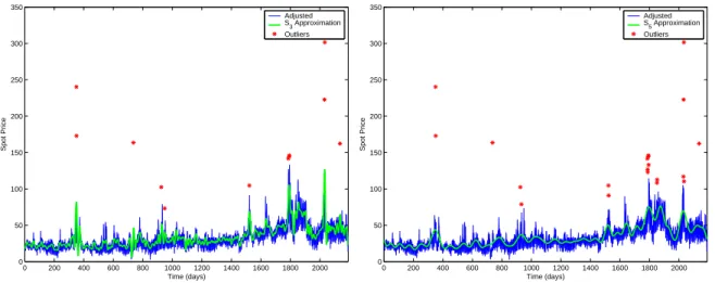
Figure 4: Time series after replacement of the spikes, S3 (left panel) andS5 (right panel)
wavelet approximations and original observations classified as outliers using the wavelet filter technique.
port – whereas the latter captures the ‘higher frequency’ detail components. Any function or signal (here: the spot price series) can be built up as a sequence of projections onto one father wavelet and a sequence of mother wavelets,
f(t) =SJ+DJ +DJ−1+...+D1, (3)
where 2J is the maximum scale sustainable by the number of observations. At the coarsest scale the signal can be estimated by SJ. At a higher level of refinement the signal can be approximated by
SJ−1 =SJ+DJ. At each step, by adding a mother wavelet Dj of a lower scale j=J −1, J −2, ..., we obtain a better estimate of the original signal. This procedure is known as lowpass filtering. Here, we use the S3 and S5 approximations, roughly corresponding to weekly (23 = 8 days) and monthly (25
= 32 days) smoothing, respectively. Once a chosen approximation (S3 orS5) is subtracted from the original price series, the outliers are identified as the observations exceeding three standard deviations of the differences. We decided to replace the outliers by their wavelet approximation. A plot of the original time series and the waveletS3andS5approximations as well as the results for outlier detection for the two approximation techniques are displayed in Figure 4.
Results
In this section we will compare the different approaches in terms of outlier detection, descriptive statistics of the remaining series and the effects of the preprocessing technique on the estimation of the seasonal pattern. In a first step we investigate the number of detected outliers, see Table 1.
The bounds for the fixed thresholds method was chosen to be 75 EUR/MWh. Obviously, de-pending on whether the technique is applied to the original or the detrended series there are substantial differences in the outcome. For the detrended series mostly observations in the years 2005 and 2006 were characterized as outliers, since the average price level was much higher in these years, see Figure 2. In total there are 50 observations replaced when the original series is considered. The respective number for the same threshold using a detrended time series only yields 19 outliers. Overall, consid-ering several years of data, it seems recommendable to choose a fixed price threshold to identify price spikes only after dealing with trends or seasonalities beforehand.
Table 1: Number of detected spikes and descriptive statistics of the series after removing the spikes. Preprocessing indicates whether the trend, the annual and/or the weekly seasonal components have been removed from the original data before identifying the spikes.
Method Preprocessing #spikes Max Mean Std Skew Kurt
Trend Year Week
Original — — — — 301.54 33.56 19.01 3.93 37.16
Fixed Threshold — — — 50 79.49 32.01 13.43 0.83 3.52
Fixed Thres. Detrend. X — X 19 108.25 32.64 14.90 1.24 5.08
Recursive Filter — — X 37 112.65 32.47 14.92 1.32 5.51
Percentage Thres. X — X 22 114.06 32.70 14.99 1.24 5.13
Wavelet Approx. S3 X X ∼ 12 132.91 33.10 16.23 1.70 7.81
Wavelet Approx. S5 X X — 20 114.06 32.78 15.14 1.27 5.18
outliers, yielding 22 observations. The comparative number for the recursive filter technique is higher and characterized 37 observations as outliers. It is notable that for the filter technique also a number of observations with a lower price level but high percentage returns were identified as price spikes. Examining the results for the wavelet decomposition techniques, we find that the S3 approximation is very close to the original time series (see the left panel of Figure 4). Thus, only a small number of observations – in total 12 – is classified as outliers. The smootherS5 approximation, on the other hand, characterizes 20 observations as outliers and yields similar results to the other techniques.
The examination of the descriptive statistics for the preprocessed series yields the following results. For all techniques, the mean of the preprocessed series is only slightly smaller than for the original observations. However, the removal of the outliers has clearly decreased the standard devia-tion, skewness and kurtosis of the remaining series. There is also a general tendency for the relationship between the number of replaced outliers and those statistics: the more extreme observations are re-placed, the more will the standard deviation, skewness and kurtosis decrease for the preprocessed series. Hence, the preprocessed series using the waveletS3 approximation yields the highest values for those statistics while they are clearly the lowest for the series that was preprocessed using the simple fixed threshold technique. The results for the other four techniques (fixed threshold detrended, recur-sive filter, percentage threshold and waveletS5) yield quite similar descriptive statistics. Interestingly, the recursive filter technique yields a preprocessed series with a slightly higher skewness and kurtosis than most of the other techniques, although a relatively high number of detected outliers has been replaced.
Finally, we compare the effects of the chosen outlier detection technique on the estimated sea-sonal pattern. We assume that the system price of electricitySt can be decomposed as the sum of a deterministic componentftand a stochastic componentYt: St=ft+Yt, t >0. In the following, we are not interested in specifying a model for the stochastic componentYt, but mainly in the estimated seasonal pattern for the differently preprocessed data. To keep the results comparable, we estimated the same seasonal pattern including a constant, trend and specified dummy variables for daily and monthly effects for all preprocessed series:
f(t) =α+β·t+d·Dday+m·Dmon. (4)
Table 2: Parameter estimates for the seasonal pattern depending on the different outlier detection techniques (* indicates significant parameter estimates at the 5% level).
Parameter Original Fixed Fixed Detr Filter Percent WaveS3 WaveS5
Constant 23.573* 22.249 22.683* 22.546* 22.998* 22.908* 22.660*
Trend 0.0158* 0.0137* 0.0150* 0.0154* 0.0151* 0.0156* 0.0152*
Tue 2.388* 0.223 1.192 1.211 0.741 1.212 0.880
Wed 0.759 1.344* 1.725* 1.217 1.381 1.414 1.436
Thu 1.156 0.949 1.2097 1.260 1.120 0.994 0.937
Fri -2.372* -1.371* -1.271 -0.919 -1.854* -1.705 -1.750*
Sat -10.277* -8.199* -8.765* -8.580* -9.135* -9.614* -9.226*
Sun -16.818* -14.750* -15.279* -15.016* -15.687* -16.146* -15.767*
Feb 0.210 1.097 1.315 1.059 1.243 0.869 1.491
Mar -1.129 0.128 -0.351 -0.313 -0.613 -0.666 -0.356
Apr -5.551* -2.601* -4.446* -4.764* -4.514* -4.896* -4.267*
May -8.862* -5.928* -7.791* -8.128* -7.846* -8.240* -7.609*
Jun -5.242* -2.661* -4.106* -4.677* -4.399* -4.595* -3.936*
Jul -0.091 -1.430 -2.198* -3.676* -2.888* -1.180 -1.839
Aug -7.021* -3.708* -5.755* -6.236* -5.840* -6.505* -5.612*
Sep -4.247* -0.898 -2.972* -3.343* -3.061* -3.549* -2.834*
Oct -5.206* -1.829* -3.929* -4.313* -4.017* -4.512* -3.792*
Nov -0.638 -0.797 -2.901* -3.327* -2.137* -1.228 -1.914
Dec -1.093 -1.144 -2.528* -4.078* -1.802 -1.787 -1.459
We find that depending on the chosen technique for outlier detection, there are significant differences between parameter estimates and also in terms of which days and months are considered to be significant. For all models, the constant and trend are highly significant. Note, however, that withβ = 0.0158 the parameter estimate for the trend component is the highest for the observations where no preprocessing of the outliers has been conducted followed by the wavelet techniqueS3 where the trend estimate isβ= 0.0156. On the other hand, the trend is estimated to be substantially lower (β = 0.0137) if the outliers are detected by a fixed threshold technique without detrending. The other methods yield estimates for the trend parameter between ofβ = 0.0150 andβ = 0.0154.
It is also noteworthy that depending on the preprocessing of the data, often quite different dummy variables for the day or month are significant at the chosen 5% level. While for all ap-proaches obviously Saturday and Sunday show a significant lower price level, for the original data also the dummy variables for Tuesday and Friday are significantly different from Monday, respectively Wednesday and Friday for the fixed threshold technique without detrending. On the other hand, preprocessing using the recursive filter technique or the waveletS3 yields only Saturday and Sunday as being significantly different from a Monday.
Similar results can be observed for the significance of dummy variables for the months. All approaches give significant parameter estimates for the months April, May, June, August and October. However, there are substantial differences for the months as well as the total number of dummy variables that yield significant estimates. While based on the simple fixed threshold preprocessing only estimates for the above mentioned months are significantly different from January, for the fixed threshold with detrending and the recursive filter approach all dummy variables for April - December are significant at the 5% level. The preprocessing using the percentage threshold technique yields significant estimates for the April - November dummy variables, while the original series and the series preprocessed with the wavelet approaches classifies April, May, June, August, September and October as significant.
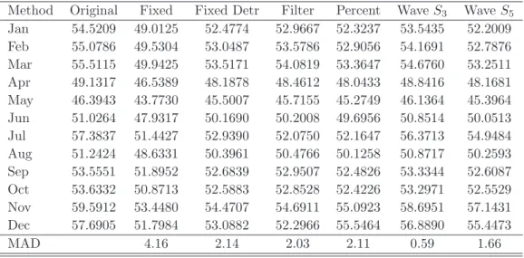
de-Table 3: Monthly price forecasts for 2007 based on the estimated seasonal pattern for the different outlier detection techniques. The last row provides the mean absolute deviation (MAD) in Euro/MWh from the forecasts for the original observations.
Method Original Fixed Fixed Detr Filter Percent WaveS3 WaveS5
Jan 54.5209 49.0125 52.4774 52.9667 52.3237 53.5435 52.2009
Feb 55.0786 49.5304 53.0487 53.5786 52.9056 54.1691 52.7876
Mar 55.5115 49.9425 53.5171 54.0819 53.3647 54.6760 53.2511
Apr 49.1317 46.5389 48.1878 48.4612 48.0433 48.8416 48.1681
May 46.3943 43.7730 45.5007 45.7155 45.2749 46.1364 45.3964
Jun 51.0264 47.9317 50.1690 50.2008 49.6956 50.8514 50.0513
Jul 57.3837 51.4427 52.9390 52.0750 52.1647 56.3713 54.9484
Aug 51.2424 48.6331 50.3961 50.4766 50.1258 50.8717 50.2593
Sep 53.5551 51.8952 52.6839 52.9507 52.4826 53.3344 52.6087
Oct 53.6332 50.8713 52.5883 52.8528 52.4226 53.2971 52.5529
Nov 59.5912 53.4480 54.4707 54.6911 55.0923 58.6951 57.1431
Dec 57.6905 51.7984 53.0882 52.2966 55.5464 56.8890 55.4473
MAD 4.16 2.14 2.03 2.11 0.59 1.66
pending on the chosen technique for outlier detection. To further illustrate the effects of the different preprocessing techniques on the seasonal pattern and possible price forecasts let us consider the follow-ing situation. Startfollow-ing with a model includfollow-ing all possible independent variables, for each preprocessed series in a backwards stepwise regression non-significant variables are excluded from the model, re-maining with a model including only significant variables. Then the estimated seasonal pattern is used to give (deterministic) price forecasts for each month in 2007. The forecast results for each of the considered methods are presented in Table 3. Note that the predicted values of the seasonal pattern should not be used as actual price forecasts, since the modeling of the stochastic component has not been considered here. However, since the system price is decomposed as the sum of the deterministic and stochastic component, significant differences in the prediction of the deterministic component will also have an substantial effect on the forecasted system price.
We find that the estimated seasonal pattern without preprocessing the data for outliers yields the highest forecasts for the deterministic part of the series for all months in 2007. On the other hand, the lowest price forecasts for each month is obtained when the simple fixed threshold technique is used for outlier detection. As the last row indicates, the average difference between these two approaches is 4.16 Euro/MWh per day. For example, the forecasted average daily price in January is almost 10% lower for the fixed threshold technique in comparison to using the original observations.The differences are smaller for the other techniques, however, the predicted price level in 2007 is still between 1.66 and 2.14 Euro/MWh lower for the outlier detection techniques fixed threshold with detrending, recursive filter, percentage threshold and waveletS5. Only the waveletS3 approximation yields similar results to the original series. Here the forecasted average price level according to the estimated seasonal pattern is only 0.59 Euro/MWh lower than for the original series. Hence, the technique that classifies the smallest number of observations as outliers also predicts the highest price level for the forthcoming months in 2007.
REFERENCES
Bhanot, K., 2000. Behavior of power prices: Implications for the valuation and hedging of financial contracts. Journal of Risk 2, 43–62.
Bierbrauer, M., Menn, C., Rachev, S., Tr¨uck, S., 2007. Spot and derivative pricing in the eex power market. Journal of Banking and Finance forthcoming.
Bierbrauer, M., Tr¨uck, S., Weron, R., 2004. Modeling electricity prices with regime switching models. Lecture Notes in Computer Science 3039, 859–867.
Borovkova, S., Permana, F., 2004. Modelling electricity prices by the potential jumpdiffusion. Proceedings of the Stochas-tic Finance 2004 Conference, Lisbon, Portugal.
Brockwell, P., Davis, R., 1991. Time Series: Theory and Methods. Springer-Verlag, New York.
Bunn, D. (Ed.), 2004. Modelling Prices in Competitive Electricity Markets. Wiley, Chichester.
Cartea, A., Figueroa, M., 2005. Pricing in electricity markets: A mean reverting jump diffusion model with seasonality. Applied Mathematical Finance 12(4), 313–335.
Clewlow, L., Strickland, C., 2000. Energy Derivatives – Pricing and Risk Management. Lacima Publications, London.
De Jong, C., 2006. The nature of power spikes: A regime-switch approach. Studies in Nonlinear Dynamics & Econometrics 10(3), Article 3.
Geman, H., Roncoroni, A., 2006. Understanding the fine structure of electricity prices. Journal of Business 79(3), 1225– 1262.
H¨ardle, W., Kerkyacharian, G., Picard, D., Tsybakov, A. (Eds.), 1998. Wavelets, Approximation and Statistical Appli-cations. Lecture Notes in Statistics 129. Springer-Verlag, New York.
Harris, C., 2006. Electricity Markets: Pricing, Structures and Economics. Wiley, Chichester.
Huisman, R., Mahieu, R., 2003. Regime jumps in electricity prices. Working paper, Rotterdam School of Management.
Kaminski, V. (Ed.), 2004. Managing Energy Price Risk: The New Challenges and Solutions, 3rd ed. Risk Books, London.
Kirschen, D., Strbac, G., 2004. Fundamentals of Power System Economics. Wiley, Chichester.
Knittel, C. R., Roberts, M. R., 2005. An empirical examination of restructured electricity prices. Energy Economics 27(5), 791–817.
Lapuerta, C., Moselle, B., 2001. Recommendations for the Dutch electricity market. The Brattle Group Report.
Lucia, J. J., Schwartz, E., 2002. Electricity prices and power derivatives: Evidence from the Nordic power exchange. Review of Derivatives Research 5, 5–50.
Percival, D., Walden, A., 2000. Wavelet Methods for Time Series Analysis. Cambridge University Press, Cambridge.
Pilipovic, D., 1997. Energy Risk: Valuing and Managing Energy Derivatives. McGraw-Hill.
Shahidehpour, M., Yamin, H., Li, Z., 2002. Market Operations in Electric Power Systems: Forecasting, Scheduling, and Risk Management. Wiley.
Stevenson, M., 2001. Filtering and forecasting spot electricity prices in the increasingly deregulated Australian electricity market. QFRC Research Paper 63, University of Technology, Sydney.
Weron, R., 2006. Modeling and Forecasting Electricity Loads and Prices: A Statistical Approach. Wiley, Chichester.
Weron, R., 2007. Market price of risk implied by Asian-style electricity options and futures. Energy Economics (forth-coming), doi:10.1016/j.eneco.2007.05.004.
Weron, R., Bierbrauer, M., Tr¨uck, S., 2004a. Modeling electricity prices: Jump diffusion and regime switching. Physica A 336, 39–48.