New Discrete Predictive Sliding Mode Control for Non Minimum Phase Systems

New Discrete Predictive Sliding Mode Control for Non

Minimum Phase Systems

Ben Mansour Houda

Research Unit: Control of Industrial Processes National Engineering School of Gabes

University of Gabes

Street of Medenine 6029 Gabes,Tunisia

Dehri Khadija

Research Unit: Control of Industrial Processes National Engineering School of Gabes

University of Gabes

Street of Medenine 6029 Gabes,Tunisia

Nouri Ahmed Said

Research Unit: Control of Industrial Processes National Engineering School of Gabes

University of Gabes

Street of Medenine 6029 Gabes,Tunisia

ABSTRACT

This paper shows the development of a Predictive Sliding Mode Controller (PSMC). The proposed controller blends the design of Sliding Mode Control (SMC) with Model Predictive Control (MPC). The combination of SMC and MPC improves the perfor-mance of these two control laws. The designed control strategy has stronger robustness and chattering reduction property to con-quer within the system uncertainties. The Predictive Sliding Mode Control strategy was improved by giving a New Predictive Slid-ing Mode Controller (NPSMC). Finally, the performances of the NPSMC, in terms of strong robustness to external disturbance and parameters variation, chattering elimination, fast convergence were judged, in comparaison with PSMC, SMC and MPC, using a non-minimum phase system.

Keywords:

Non minimum phase systems, Sliding mode control, Model pre-dictive control, Prepre-dictive sliding mode control, Chattering phe-nomenon.

1. INTRODUCTION

The classical Bode integral theorems provide unique relation-ships between the amplitude and the phase of the frequency re-sponse for a minimum phase system. A plant with dead-time or with a right-half plane zero is called non-minimum phase sys-tem as these relationships are then no longer valid [1]. It is well known that such plants are not easy to control because they have an initial inverse response to step input in the opposite direc-tion to the steady state [2]. In some sense all practical discrete time systems are non-minimum phase. The presence of unstable zero in a process transfer function is thus identified as being re-sponsible for its difficult dynamic behavior; it is also the source of a considerable amount of difficulty in controller design. An other aspect of controlling a process with unstable zero is the problem of instability, which arises in order to achieve high per-formance when the controller contains an inverse of the process model [3, 4].

Model Based Predictive Control (MPC) has become one of the most popular control methodologies both in industry and academia [7]. Furthermore, the instability problems applying

Model Predictive Control to non minimum phase systems have been reported in literature [4, 8], showing that the non-minimum phase systems produce instability when the control horizon and the maximum predictive horizon are equal to1, while [9, 10] demonstrated that this can be tuned to have stable behavior with unstable zero in the Single Input Single Output (SISO) case. MPC has instability problems because, for non-minimum phase plants, the controller achieves the optimal output by canceling the plant zeros, including the unstable zero, which leads to loss of internal stability of the feedback system [11, 12].

On the other hand, Sliding Mode Control (SMC) is a technique derived from Variable Structure Control (VSC) which was stud-ied originally by Utkin [13]. For a broad class of systems, this kind of control is particulary appealing due to its ability to deal with nonlinearities, parameter uncertainties and disturbances. However, undesired chattering produced by the high frequency switching of the control may be considered as a problem for im-plementing the sliding mode control methods to some real appli-cations [20].

illus-trated. Section4describes the synthesis of the new Predictive Sliding Mode Controller, with a simulation example. In section 5, the advantages of the presented controllers are verified by a non minimum phase system with disturbances and parameter variations. These results are compared with Sliding mode Con-troller and Model Predictive ConCon-troller. Finally, section6draws conclusions of the paper.

2. BASIC CONCEPTS

2.1 System description and preliminaries

Consider the following uncertain discrete time system [15]:

x(k+ 1) = (A+ ∆A)x(k) + (B+ ∆B) (u(k) +v(k))

y(k) =Hx(k) +Du(k)

(1) Wherex(k)∈Rn_{is the state vector andu(k)∈Ris the scalar}

input control. The matricesA,B, H andD are the nominal model matrices with adequate dimensions. The parameter uncer-tainties are given by∆Aand∆B.v(k)∈Ris the disturbance input.

The system (1) can be written in the following form:

x(k+ 1) =Ax(k) +Bu(k) +w(k)

y(k) =Hx(k) +Du(k) (2)

with

w(k) = ∆Ax(k) + ∆Bu(k) + (B+ ∆B)v(k) (3)

2.2 Sliding mode control

In this section, we present the control law based on the sliding mode. The sliding function is defined as:

s(k) =Cx(k) (4)

whereC∈R1×n_.

A necessary and sufficient condition assuring sliding motion and convergence to the sliding surface is:

|s(k+ 1)|− |s(k)|<0 (5)

According to sliding mode function (4), the sliding mode value at the instant(k+ 1)can be obtained as:

s(k+ 1) =Cx(k+ 1)

s(k+ 1) =C[Ax(k) +Bu(k) +w(k)]

s(k+ 1) =C[Ax(k) +Bu(k)] +Cw(k)

(6)

If there are no disturbances, the sliding function (4) value at time (k+p)[17] is:

s(k+p) =Cx(k+p)

s(k+p) =CAp_{x(k) +} p

P

j=1

CAj−1_Bu(k+p−j) (7)

wherek∈Zandp∈N.

To obtain the desiral performances, such as strong-robustness, fast convergence and chattering elimination, we introduced a reaching law to ensure the convergence of the sliding function

s(k)to zero.

To ensure a quasi-sliding mode, the sliding mode function must verify the reaching law [15]:

s(k+ 1) =s(k)−msgn(s(k)) (8) where sgn is the signum function defined as:

sgn (s(k)) :=

−1 if s (k)<0 1 if s (k)>0

andmis the discontinuous term magnitude. Using the last equation and equation(6), we obtain:

s(k+ 1)−s(k) =Cx(k+ 1)−s(k)

s(k+ 1)−s(k) =CAx(k) +CBu(k)−s(k)

s(k+ 1)−s(k) =s(k)−msgn(s(k))−s(k)

s(k+ 1)−s(k) =msgn(s(k))

Then, the control law can be calculated as:

u(k) = (CB)−1_{[s(k)−CAx(k)−msgn(s(k))] (9)}

2.3 Model Predictive control

Model Based Predictive Control (MPC) has been successfully implemented in many industrial applications, showing a good performance [4].

MPC does not designate a specific control strategy but a very ample range of control methods, which make an explicit use of a model of the process to obtain the control signal by minimiz-ing an objective function. The synthesis of predictive control law consist of three steps. The first step is to predict the process out-put at future time instants. The second step is to calculate control sequence minimizing an objective function. The third step is to consider that the control law is the first element of control se-quence. The basic idea of MPC is to calculate a sequence of fu-ture control signals in such a way that it minimizes a multistage cost function [4, 22]:

J(N0, N, M) =

N

P

j=N0

q(j) [yr(k+j)− y(k+j/k] 2

+

M

P

j=1

λ(j) [u(k+j−1)]2

wherey(k+j/k)is an optimum j-step ahead prediction of the system output on data up to timek,N0

andNare the minimum and maximum costing horizon,M is the control horizon,q(j) andλ(j)are the weighting sequences, andyr(k+j)is the future

reference trajectory.

The objective of MPC is to compute the future control sequence

u(k),u(k+ 1),...in such a way that the future plant outputy(k+

j)is driven close toyr(k+j)by minimizing the quadratic cost

functionJ(N0_{, N, M)[4, 22].}

3. PREDICTIVE SLIDING MODE

CONTROLLER

3.1 Synthesis of Predictive Sliding Mode controller

In this section, we consider the sliding mode control problem for system (1), taking reaching law (8). The reference sliding mode trajectory is chosen as [17, 18]:

sr(k+p) =sr(k+p−1)−msgn(sr(k+p−1))

sr(k) =s(k) (10)

The objective is to design a sliding mode predictive control, using equation (6) and consider thatw(k)is equal to zero, the sliding function at instant(k+p)can be written as:

s(k+p) =CAp_{x(k) +} p

P

j=1

CAj−1_Bu(k+p−j)

wherek∈Nandp∈N.

Therefore, the predictive sliding mode value of timekon time (k−p)can be deduced:

s(k/k−p) =CAp_{x(k−p) +} p

P

j=1

CAj−1_Bu(k−j)

(11)

Equation (11) can be described in vector form as follows:

where

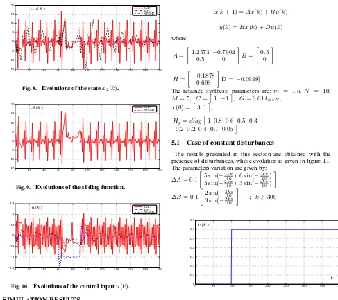
Sp(k+ 1) = [s(k+ 1), s(k+ 2), ..., s(k+N)]T U(k) = [u(k), u(k+ 1), ..., u(k+M−1)]T

Γ =h(CA)T (CA2₎T

... CANTiT

Ω =



        

CB 0 ... ... 0

CAB CB ... ... 0

. . ... ... .

. . ... ... .

CAM−1_{B CA}M−2_{B ... CAB CB}

. . ... . .

CAN−2_{B CA}N−3_{B ... CA}N−M_{B CA}N−M−1_B

CAN−1_{B CA}N−2_{B ... CA}N−M+1_{B CA}N−M_B



        

With N is the prediction horizon, M is control horizon and the minimum costing horizonN0_{is chosen equal to1.}

In practice, to make correction to the future predictive sliding mode values(k+p), we introduce the error between practi-cal sliding mode values(k)and predictive sliding mode value

s(k/k−p). Therefore, the output of sliding mode prediction ˜

sp(k+p)is given as follows:

˜

sp(k+p) =s(k+p) +hpe(k)

˜

sp(k+p) =CApx(k) + p

P

j=1

CAj−1_Bu(k+p−j)

+hpe(k)

(13)

Wheree(k) =s(k)−s(k/k−p)andhpis a correct coefficient.

Rewrite Equation (13) in vector form: ˜

Sp(k+ 1) =Sp(k+ 1) +HpE(k) (14)

where ˜

Sp(k+ 1) = [˜sp(k+ 1),s˜p(k+ 2), ...,˜sp(k+N)] T

Hp=diag[h1, h2, ..., hN]

E(k) =S(k)−Smp(k)

S(k) = [s(k), s(k), ..., s(k)]_1×N

Smp(k) = [s(k/k−1), s(k/k−2), ..., s(k/k−N)]T

The following corresponding optimization cost function is de-fined [19]:

jp= N

X

j=1

qj[˜sp(k+j)−sr(k+j)] 2

+

M

X

l=1

gl[u(k+l−1)] 2

(15) wheresr(k+j)is the sliding mode reference trajectory,qjand glare weight coefficients.

In order to simplify the synthesis of the controller, we consider(qj= 1)andgl=g. So, The following corresponding

optimization cost function is written as:

jp= N

X

j=1

[˜sp(k+j)−sr(k+j)]2+ M

X

l=1

g[u(k+l−1)]2

(16) Rewrite Equation(16) in vector form:

Jp=

S˜p(k+ 1)−Sr(k+ 1)

+kU(k)k 2

G=

[Γx(k) + ΩU(k) +HpE(k)−Sr(k+ 1)]

T [Γx(k) +ΩU(k) +HpE(k)−Sr(k+ 1)] +U(k)TGU(k)

(17)

where

Sr(k+ 1) = [sr(k+ 1), sr(k+ 2), ..., sr(k+N)] T

G= [g, g, ..., g]

The optimal sequence of control is obtained by minimizing the cost functionJp:

∂Jp ∂U(k) = 0

Then, this sequence can be calculated as:

U(k) =−(ΩT_{Ω +G)}−1_ΩT_{[Γx(k) +H}

pE(k)−Sr(k+ 1)]

(18) Because of rolling optimization, only the present control input signal is implemented, the next time control signalu(k+ 1)will be calculated recursively by the control law.

3.2 Simulation example

The behavior, of the PSMC is illustrated by a simulation exam-ple. Let’s consider the following system [17]:

x(k+ 1) =Ax(k) +Bu(k) +w(k)

where:

A=

1 0.01

−0.651 0.797

B=

0 0.731

The sampling periodT is chosen, according to the system’s dynamics, equal to0.01s.

For the Predictive Sliding Mode controller, choosing

G = 0.001∗IM×M. C is designed as C =

3 1 and setting the initial period valuesx(0) =1 0.5

.

Select the predictive horizon N = 10, the control horizon

M= 5and the correct coefficient matrix:

Hp=diag

1 0.8 0.6 0.5 0.3 0.2 0.2 0.4 0.1 0.5

Satisfying the robustness condition, the discontinuous term magnitudemis chosen as follow:

m= 3 if 48<k<92

m= 0.02 else

The results presented in this section are obtained with the pres-ence of disturbances, whose evolution is given in figure1, and parameters variation are given by:

∆A= 0.5

0 0

3 sin(−2kπ

10) 3 sin(− 2kπ

10 )

∆B= 0.5

0 sin(−2kπ

10

0 20 40 60 80 100 120 140 160 180 200 0

0.1 0.2 0.3 0.4 0.5 0.6 0.7 0.8 0.9 1

k d(k)

The simulation results of PSMC are illustrated in figure2to fig-ure5. These figures are a comparaison between the results given by PSMC, SMC and MPC. In fact, figure2and3show the evo-lution of the statex1(k)andx2(k). Figure4presents the

evo-lution of the sliding surface. The evoevo-lution of the inputu(k)is presented in figure5.

0 20 40 60 80 100 120 140 160 180 200

−1.5 −1 −0.5 0 0.5 1 1.5 2 2.5

PSMC SMC MPC x1(k)

k

Fig. 2. Evolutions of the statex1(k).

0 20 40 60 80 100 120 140 160 180 200 −15

−10 −5 0 5 10 15 20

PSMC SMC MPC x2(k)

k

Fig. 3. Evolutions of the statex2(k).

0 20 40 60 80 100 120 140 160 180 200 −15

−10 −5 0 5 10 15 20

PSMC SMC S(k)

k

Fig. 4. Evolutions of the sliding function.

These figures prove that the control law, given by Predictive Slid-ing Mode Controller, can eliminate the chatterSlid-ing and force the states to converge to zero better than Sliding Mode Controller and Model Predictive Controller. But, it is still not able to reject the constant disturbances perfectly.

4. NEW PREDICTIVE SLIDING MODE

CONTROLLER

4.1 Synthesis of New Predictive Sliding Mode controller

To ameliorate the performances in term of rejecting constant and periodic disturbances, we propose in this section a New Predictive Sliding Mode Controller (NPSMC).

The optimal control problem is calculated, now, using a cost

0 20 40 60 80 100 120 140 160 180 200 −1.5

−1 −0.5 0 0.5 1 1.5

PSMC SMC MPC u(k)

k

Fig. 5. Evolutions of the control inputu(k).

function penalizing deviation of the controlled variables as well as variations in the control signal. So the NPSMC block diagram can be represented as follow: The objective is to design the

Model

Predictive

Control

ΔU

°

_p

S

Sr

Sliding Mode

Control

C

X

Fig. 6. NPSM Controller block diagram.

sliding mode predictive control, or we have :

s(k+p) =CAp_{x(k) +} p

P

j=1

CAj−1_Bu(k+p−j)

wherek∈Zandp∈N.

The sliding function at the instancek+ 1,k+ 2andk+ 3can be written as:

s(k+ 1) =Cx(k+ 1)

= CAx(k) + CB(u(k)−u(k−1)) + CBu(k−1) = CAx(k) + CBδu(k) + CBu(k−1)

s(k+ 2) =Cx(k+ 2) = CAx(k + 1) + CBu(k + 1)

= CA2x(k) +CBδu(k+ 1) +CABδu(k)+CBδu(k) +CBu(k−1) + CABu(k−1)

= CA2x(k) +CBδu(k+ 1) +C(A+ 1)Bδu(k) +C(A+ 1)Bu(k−1)

s(k+ 3) =Cx(k+ 3)

= CA [A[Ax(k) +Bu(k)]] +CABu(k+ 1) +CBu(k+ 2) = CA3_{x(k) +CBδu(k+ 2) +C(A+ 1)Bδu(k+ 1)}

+C(A2+A + 1)Bδu(k) + C(A2+A + 1)Bu(k−1)

Then,s(k+p)can be calculated as:

s(k+p) =CAp_{x(k) +CBδu(k+p−1)}

+C(A+ 1)δu(k+p−2) +· · ·+C

p−1 P

j=0

Aj

Bδu(k)

+C

p−1 P

j=0

Aj

Bu(k−1)

(19) where δu(k) =u(k)−u(k−1)Equation (19) can be described in vector form as follows:

where

Sp(k+ 1) = [s(k+ 1), s(k+ 2), ..., s(k+N)] T

Sp(k) = [s(k), s(k+ 1), ..., s(k+N−1)] T

∆U(k) = [δu(k), δu(k+ 1), ..., δu(k+M−1),0, ...,0]T

Γ =h(CA)T (CA2₎T

... CANTiT

ΩF ₌

            

CB 0 ... ... 0

C(A+I)B CB ... ... 0

. . ... ... .

. . ... ... .

C

M−1 P

j=0

Aj

B ... ... C(A+I)B CB

. . ... . .

C

N−1 P

j=0

Aj

B ... ... C

N−M−1 P

j=0

Aj

B C

N−M

P j=0 Aj B             

With N is prediction horizon, M is control horizon and the mini-mum costing horizonN0is chosen equal to1.

and

ΩP =

            CB .. . C

M−1 P j=0 Aj B .. . C

N−1 P j=0 Aj B            

In practice, to make correction to the future predictive sliding mode values(k+p), we introduce the error between the practical sliding mode values(k)and the predictive sliding mode value

s(k/k−p). Therefore, the output of sliding mode prediction ˜

sp(k+p)is given as follows:

˜

sp(k+p) =s(k+p) +hpe(k)

˜

sp(k+p) =CApx(k) +CBδu(k+p−1)

+C(A+ 1)δu(k+p−2) +· · ·+C

p−1 P

j=0

Aj

Bδu(k)

+C

p−1 P

j=0

Aj

Bu(k−1)+hpe(k)

(21) Wheree(k) =s(k)−s(k/k−p)andhpis a correct coefficient.

Rewrite Equation (21) in vector form: ˜

Sp(k+ 1) =Sp(k+ 1) +HpE(k) (22)

where ˜

Sp(k+ 1) = [˜sp(k+ 1),s˜p(k+ 2), ...,˜sp(k+N)] T

Hp=diag[h1, h2, ..., hN]

E(k) =S(k)−Smp(k)

S(k) = [s(k), s(k), ..., s(k)]₁×N

Smp(k) = [s(k/k−1), s(k/k−2), ..., s(k/k−N)] T

The following corresponding optimization cost function is de-fined:

jp= N

X

j=1

qj[˜sp(k+j)−sr(k+j)] 2

+

M

X

l=1

gl[δu(k+l−1)] 2

(23)

wheresr(k+ 1)is the sliding mode reference trajectory,qjand glare weight coefficients.

In order to simplify the synthesis of the controller, we consider (qj= 1)andgl=g. So, The following corresponding

optimiza-tion cost funcoptimiza-tion is written by:

jp= N

X

j=1

[˜sp(k+j)−sr(k+j)] 2

+

M

X

l=1

g[δu(k+l−1)]2

(24) Rewrite Equation(24) in vector form:

Jp=

S˜p(k+ 1)−Sr(k+ 1)

2

+k∆U(k)k2_G

=Γx(k) + ΩF_{∆U(k) + Ω}P_{u(k−1) +H} pE(k)

−Sr(k+ 1)]T

Γx(k) + ΩF_{∆U(k) + Ω}p_u(k−1)

+HpE(k)−Sr(k+ 1)] + ∆U(k)TG∆U(k)

(25)

where

Sr(k+ 1) = [sr(k+ 1), sr(k+ 2), ..., sr(k+N)] T

G= [g, g, ..., g]

Let ∂Jp

∂∆U(k) = 0, the optimal law can be obtained:

∆U(k) =−((ΩF₎T_ΩF_+G)−1_(ΩF₎T_{[Γx(k) +H} pE(k)

−Sr(k+ 1)]

(26) Because of rolling optimization, only the present increment of control input signal is implemented, the next time increment of control signalu(k+ 1)will be calculated recursively by the con-trol law.

δu(k) = [1,0, ...0]T∆U(k) (27) So, we have:

u(k) =u(k−1) +δu(k) (28)

4.2 Simulation example

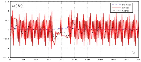
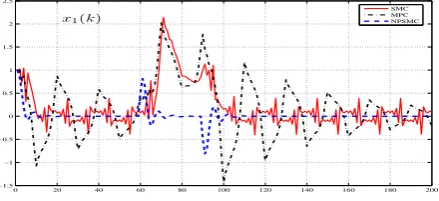
To improve the behavior of the NPSMC, we kept the same sim-ulation example of the last section. Compared to SMC and MPC , the simulation results of NPSMC are illustrated in figure7to figure10.

In fact, figure7and 8show, respectively, the evolution of the statesx1(k)and x2(k). Figure9presents the evolution of the

sliding surface. The evolution of the inputu(k)is presented in figure10.

0 20 40 60 80 100 120 140 160 180 200 −1.5 −1 −0.5 0 0.5 1 1.5 2 2.5 SMC MPC NPSMC

x1(k)

Fig. 7. Evolutions of the statex1(k).

0 20 40 60 80 100 120 140 160 180 200 −15

−10 −5 0 5 10 15 20

SMC MPC NPSMC

x2(k)

Fig. 8. Evolutions of the statex2(k).

0 20 40 60 80 100 120 140 160 180 200

−15 −10 −5 0 5 10 15 20

SMC NPSMC

S(k)

Fig. 9. Evolutions of the sliding function.

0 20 40 60 80 100 120 140 160 180 200

−1.5 −1 −0.5 0 0.5 1 1.5

SMC MPC NPSMC

u(k)

Fig. 10. Evolutions of the control inputu(k).

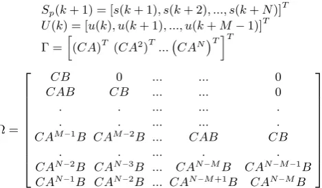
5. SIMULATION RESULTS

To evaluate the robustness of the two control laws equations (18) and equation (26), we consider the isothermal Van de Vussen systems [11]. this system involves series and parallel reactions and is governed by the following equations:

Ca

dt =−k1Ca−k3Ca2+ (Cain−Ca)FV C_b

dt =k1Ca−k2CbVF

(29)

The desired output is the concentration of B, Cb [mol/l],Ca

and Cain are the concentrations of A [mol/l] in the reactor

and in the feed respectively, the manipulate input, F is the dilution rate [l/min], V is the volume [l], and the rate con-stants are given by k1 = 5/6[min−1], k2 = 5/3[min−1],

k3= 1/6[mol/litermin][11].

Above no linear, non minimum phase process has been used to show the controller performance. After linearizing model (29) about the operating point the physical model gives the following transfer function (30). The discretization has been made with ampling rateTe= 0.2

y(k) = −0.0939 + 0.1745z −1

1−1.2573z−1_{+ 0.3951z}−2u(k−1) (30)

The state space representation of the isothermal Van de Vussen systems is given as follows:

x(k+ 1) =Ax(k) +Bu(k)

y(k) =Hx(k) +Du(k)

where:

A=

1.2573 −0.7902

0.5 0

B=

0.5 0

H =

−0.1878 0.698

D = [−0.0939]

The retained synthesis parameters are:m = 1.5, N = 10,

M= 5, C=1 −1

, G= 0.01IN×N, x(0) =3 1,

Hp=diag

1 0.8 0.6 0.5 0.3 0.2 0.2 0.4 0.1 0.05

5.1 Case of constant disturbances

The results presented in this section are obtained with the presence of disturbances, whose evolution is given in figure11. The parameters variation are given by:

∆A= 0.1

5 sin(−2kπ

10) 6 sin(− 2kπ

10)

3 sin(−2kπ

10) 3 sin(− 2kπ

10)

∆B= 0.1

2 sin(−2kπ 10

3 sin(−2kπ 10

; k≥300

0 50 100 150 200 250 300 350 400 0

0.1 0.2 0.3 0.4 0.5 0.6 0.7

k v(k)

Fig. 11. Evolutions of disturbances.

The comparaison between the NPSMC, PSMC, SMC and MPC are given in figures12to15. Figure12and figure13illustrate respectively the evolution of statesx1(k)andx2(k). The

evolu-tion of the sliding funcevolu-tion is shown in figure14. Finally, figure 15shows the evolution of the control inputu(k).

0 50 100 150 200 250 300 350 400 −1

0 1 2 3 4

MPC PSMC SMC NPSMC

k x1(k)

Fig. 12. Evolutions of the statex1(k).

0 50 100 150 200 250 300 350 400 −0.5

0 0.5 1 1.5 2

MPC PSMC SMC NPSMC x2(k)

k

Fig. 13. Evolutions of the statex2(k).

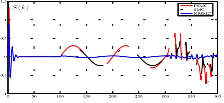
0 50 100 150 200 250 300 350 400 −1

−0.5 0 0.5 1 1.5

PSMC SMC NSMC S(k)

k

Fig. 14. Evolutions of the sliding function.

0 50 100 150 200 250 300 350 400 −2.5

−2 −1.5 −1 −0.5 0 0.5 1

MPC PSMC SMC NPSMC u(k)

k

Fig. 15. Evolutions of the control inputu(k).

disturbances, hard parameters variation, but also, in eliminating chattering.

5.2 Case of periodic disturbances

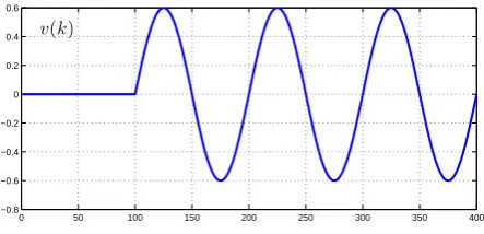
The results presented in this section are obtained with the presence of disturbances, whose evolution is given in figure16, and parameters variation are given by:

∆A= 0.1

5 sin(−2kπ

10) 6 sin(− 2kπ

10)

3 sin(−2kπ

10) 3 sin(− 2kπ

10)

∆B= 0.1

2 sin(−2kπ 10

3 sin(−2kπ 10

; k≥300

The states response, the sliding mode function and the control input,with PSMC, NPSMC, SMC, and MPC are given, respec-tively, in Figures17to20.

.

A comparaison between the NPSMC, PSMC, SMC and MPC re-veals that the use of the new control strategy (NPSMC) reduce the chattering problem effectively (k≥300).

Furthermore, the results obtained prove the capability of the pro-posed control law to reject periodic disturbances.

0 50 100 150 200 250 300 350 400

−0.8 −0.6 −0.4 −0.2 0 0.2 0.4 0.6

v(k)

Fig. 16. Evolutions of disturbances.

0 50 100 150 200 250 300 350 400 −3

−2 −1 0 1 2 3

MPC PSMC SMC NPSMC x1(k)

k

Fig. 17. Evolutions of the statex1(k).

0 50 100 150 200 250 300 350 400

−2 −1.5 −1 −0.5 0 0.5 1 1.5 2

MPC PSMC SMC NPSMC

k x2(k)

Fig. 18. Evolutions of the statex2(k).

6. CONCLUSION

The predictive sliding mode controller, presented in this paper, combines the design technique of SMC and MPC. A predictive sliding mode control strategy is proposed and a discrete-time reaching law is improved by applying a predictive sliding surface and a reference trajectory. It is shown that mixing both control techniques gives a new controller with a better robustness proper-ties. To ameliorate the performances of the PSMC, we introduce the NPSMC whose performance was judged using a non mini-mum phase system. In fact, The New Predictive Sliding Mode controller can guarantee desired performance, such as chattering elimination, fast convergence, strong robustness to constant and periodic disturbances and parameters variation.

7. ACKNOWLEDGEMENT

”This work was supported by the Ministry of the Higher Educa-tion and Scientific Research in Tunisia”

8. REFERENCES

[1] D.W. Clarke,Self-tuning control of Non minimum-phase sys-tems, Automatica, Vol. 20, no.5, pp. 501-517, 1984. [2] B.A. Ogunnaike, W.H. Ray,Process Dynamics, Modeling

0 50 100 150 200 250 300 350 400 −1

−0.5 0 0.5 1 1.5

PSMC SMC NPSMC

S(k)

k

Fig. 19. Evolutions of the sliding function.

0 50 100 150 200 250 300 350 400

−2.5 −2 −1.5 −1 −0.5 0 0.5 1 1.5

MPC PSMC SMC NPSMC

u(k)

k

Fig. 20. Evolutions of the control inputu(k).

[3] B.R. Holt, M. Morari,Design of resilient processing plant-vi. the effect of rignt half plane zeros on dynamic resilience, Chemical Engineering Science, Vol. 40, nO.1, pp. 59-74, 1985.

[4] D.W. Clarke, M. Mohtadi, P.S. Tuffs,Generalized Predictive Control: Part i: The basic Algorithm, Automatica, Vol. 23, nO.2, pp. 137-148, 1987.

[5] E.F. Camacho, C. Bordon,Model Predictive Control, (2nd edition). London: Springer.

[6] R.J. Culi, C. Bordon,Iterative nonlinear model predictive control. Stability, robustness and applications, Control En-gineers Practice,, Vol. 16, pp. 1023-1034, 2008.

[7] A. Bemporad, M. Morari, Control of systems integrating logic, dynamics and constraints, Automatica, Vol. 35, pp. 407-427, 1990.

[8] J.M. Maciejowski, Predictive Control with Constraints, Prentice Hall, Harlow, 2011.

[9] D.W. Clarke, M. Mohtadi, P.S. Tuffs,Generalized Predictive Control: Part ii: Extensions and interpretation, Automatica, Vol. 23, nO.2, pp. 149-160, 1987.

[10] R.R. Bitmead, M. Gevers and V. Wertz, Adaptative op-timal Control: The thinking man’s GPC, Prentice Hall, Brunswick, 1990.

[11] W.G. Gabin, E.F. Camacho,Sliding mode model based pre-dictive control for non minimum phase systems, European control conference, Cambridge UK, 2003.

[12] W.G. Gabin, D.Zambrano and E.F. Camacho,Sliding mode predictive control of a solar air conditionning plant, Control Engeneering Practice, Vol.17, pp. 652-663 2009.

[13] V.I. Utkin, Sliding modes in control and optimization, Spring-Verlag, Moscow, 1981.

[14] M.L. Corradini and G. Orlando,A VSC algorithme based on generalized predictive control, Automatica, Vol. 33, pp. 927-932, 1997.

[15] W. Gao, Y. Wang, A. Homaifa, Discrete-time variable structure control systems, IEEE Transactions on Industrial Electronics, Vol. 42, No. 2, pp. 117-122, 1995.

[16] J. Zhou,Z.Liu and R. Pei,A new non linear model Predic-tive control scheme for discrete time systems based on slid-ing mode control, American Control Conference Arlington, pp. 3079-3084 2001.

[17] H. Ben Mansour, A. S. Nouri,Discrete Predictive Sliding Mode control of uncertain systems, Proccedings of the 9th International Multi-Conference on System, Signals and De-vices, 2012.

[18] H. Ben Mansour, N. Abdennebi, A. S. Nouri,A New Slid-ing Function for Discrete Predictive SlidSlid-ing Mode control of time delay systems, 13th International conference on Sci-ences and Techniques of Automatic control and computer engineering, 2012.

[19] M. De La Parte, O. Camacho, E. Camacho,Developement of a GPC-based sliding mode controller, ISA Transaction, Vol. 41, pp. 19-30, 2002.

[20] M. Mihoub , A.S. Nouri, R.Ben Abdennour,Real-time ap-plication of discrete second order sliding mode control to a chemical reactor, Control Engineering Practice, pp. 1-7, 2009.

[21] A. Cavallo, C. Natale,High-order sliding control of me-chanical systems: theory and experiments, Automatica, Vol. 12, pp. 1139-1149, 2004.

[22] D. Clarke, R. Scattolini,Constrained receding horizon pre-dictive control, IEEE Trans. Automat. Contr., Vol. 23, No. 2, pp. 347-354, 1991.