http://dx.doi.org/10.4236/jep.2015.68081
Estimation of Future Generated
Amount of E-Waste in the
United States
Shoou-Yuh Chang, Godwin Appiah Assumaning, Yassir Abdelwahab
Department of Civil and Environmental Engineering, North Carolina A&T State University, Greensboro, NC, USAEmail: [email protected], [email protected], [email protected]
Received 14 July 2015; accepted 25 August 2015; published 28 August 2015
Copyright © 2015 by authors and Scientific Research Publishing Inc.
This work is licensed under the Creative Commons Attribution International License (CC BY).
http://creativecommons.org/licenses/by/4.0/
Abstract
Electrical and electronic equipment waste, or e-waste, is one of the fastest growing waste streams in the United States. The main objective of this study is to estimate the future quantities of e-waste of thirteen selected electric and electronic products in the United States in 2025. To estimate the future amount of e-waste, the authors performed a material flow analysis. The model inputs are historical and future product sales data and the product’s average life span. Sensitivity analysis was constructed to evaluate the effect of the model inputs (average life span and future sales data) in the generation of e-waste. The results show that about 1.0835 billion units will reach their end of life (EOL) in 2025; cell phone devices are the highest occurring product among the thirteen se-lected products and weighted for about 66.0% of units of the total amount, followed by computer products at 18.0%, TV products at 11.6%, computer monitors at 1.7%, hard copy peripherals (HCP) at 1.6%, and computer accessories at 1.0%. The sensitivity analysis shows that the product life span has an effect on the e-waste generation amounts from the products under study, while the sensitivity analysis of forecasted future sales indicates that the generated waste will increase or decrease according to the sales trend.
Keywords
E-Waste, Material Flow Analysis, United States, Estimation
1. Introduction
metals found in US landfills come from electronic discards. Managing e-waste has become a major challenge in many developing countries. It is expected that the amount of e-waste will increase between 16% - 28% every year [1]. The challenge faced in e-waste management is not only the growing quantities of waste but also the complexity of e-waste. E-waste is one of the most complex waste streams because of the wide variety of
prod-ucts ranging from mechanical devices to highly integrated systems and rapid change in the prodprod-ucts’ design [2].
Electrical and electronic products are an integration of numerous modern technologies and are composed of many different materials and components. The composition of the electrical waste and electronic equipment
de-pends on each item that composes it; it can be divided into six categories [3].
1) Iron and steel, used in cabinets and frames.
2) Non-ferrous metals, above all copper used in cables.
3) Glass, used in screens and displays.
4) Plastic, used in cabinets, cables coating and circuit boards.
5) Electronic components mounted on circuit boards.
6) Others, such as rubber, wood, ceramics, etc.
E-waste accounts for approximately 1% - 2% of the municipal solid waste stream in the United States. But it
garners a great deal of interest for several reasons [4].
1) Rapid growth and change in this product sector, leading to a constant stream of new product offerings and a
wide array of used products needing appropriate management.
2) The intensive energy and diverse material inputs that go into manufacturing electronic products represent a
high degree of embodied energy and scarce resources, many of which can be recovered.
3) The presence of substances of concern in some electronics, particularly older products, which merit greater
consideration for safe, EOL management.
4) The opportunities for resource conservation and recovery through improved collection and recycling of
elec-tronics.
Consumer electronics have become increasingly popular and culturally important over the past several dec-ades, changing how we communicate, entertain ourselves, get information, and the speed with which we do so. As the nature, use, and number of electronic products change over time, patterns of sales, storage, and EOL management also change. Waste managers, manufacturers, and policymakers need reliable and current
informa-tion to inform and improve the management of used electronics [4].
Traditionally, there have been several approaches to estimate or quantify the amount of e-waste generated in developing countries. The practical way is to roughly estimate the waste amount based on the sales and the life span of the products, which is known as the market supply model (Carnegie Mellon method). The market supply method, which requires the historical sales data combined with the average life span of the products, is widely
used to estimate e-waste [1] [2] [5] [6], which is used in this study. There are other models used to estimate
e-waste amounts, such as the time step model, leaching model, market supply model, distribution delay, and stock and life span model, and each model requires different input data
In the present situation, there is still a need for more accurate information on the electrical and electronic equipment put on the market as well as the quantity of e-waste generated and disposed each year. The situation is more or less the same in all countries. There are at least two factors influencing the amount of the e-waste.
1) The quantity of the products put on the market (sales data).
2) Life span of the product.
2. Literature Review
The authors developed a mathematical framework to estimate the future outflows and infrastructure needed to
recycle personal computer systems in California [2]. In addition to that, the authors estimated the total cost of e-
waste recycling in California. He used the time-series material flow analysis model in the study. The study indi-cated that the inflow pattern and amount had a great impact on the outflow pattern and amount for computer systems. According to the authors the availability of accurate data had a great impact in the model result, espe-cially the life span of the products. The authors showed that the State of California has to establish more recov-ery facilities after the year 2005 in order to recycle the computer systems in a proper way.
a material flow analysis for seven selected items: refrigerators, freezers, washing machines, televisions, audio systems, computers, and cell phones, the authors used this metrics, because they are the most representative of the WEEE considering, the weight, sales volume, lifetime, presence and importance of hazardous substances. The model assumptions were based on two types of markets: mature market for products such as refrigerators, freezers, washing machines, televisions, and audio systems and non-mature market for computers and cell phones because of the technological changes affecting life span. The model inputs were sales data and the stock in use for the products. The model result shows that the average life span is not constant for such products as computers and cell phones.
A time-step model developed to estimate the generation e-waste amount in Japan by [8]. The model inputs
were average life span and the product’s weight. The result of this study indicated that the waste weight of four of the items, air conditioners, collecting cathode ray tube (CRT) TV sets, refrigerators, and washing machines were larger than any of the other items in this study. There are some items for which the stock increased or de-creased: for example, the waste amount of items such as CRT TVs, VCRs, and CRT displays was larger than the domestic shipment amount, and their stock decreased. This is due to drastic replacement by liquid-crystal dis-play (LCD) or plasma disdis-play TVs and DVD dis-players during that period. On the other hand, the waste amount of items such as DVD players, LCD displays, and printers was smaller than the domestic shipment amount. This is because these items have been growing in volume.
An approach and methodology constructed to estimate the future outflows of the electrical and electronic
waste in India by [1]. He used a time series, multiple life span, and EOL model. The model estimates future
e-waste generation by modeling the electrical and electronic equipment usage and disposal. The result of the study indicates that the influence of WEEE estimated is the inflow amount (sales data) and the first-user deci-sion. In addition to that, the accuracy of the model result is dependent on how accurate the available data are and the assumptions on the average life span of the products.
A paper published by [9] discussed two different approach types of material flow models: delay model and
leaching model. The leaching model is where the estimation of the present outflow can be derived from the size of the present stock. This means that the amount of outflow is considered to be equal to a fraction of the stock. The advantages of this model are that it does not require more data and it is easy for calculation. In the delay model (dynamic model), the outflow in a certain year is equal to or a function of the inflow in the past because the material is disposed after it has worn out, gone out of fashion, or is no longer compatible with other products. The model required the life span of the product and historical data.
Material flow analysis for five pieces of household electrical and electronic equipment, namely televisions, washing machines, air conditioners, refrigerators, and personal computers to constructed to estimate the e-waste
quantity by [10]. The result shows an increase in e-waste generation from both households and business sectors
in study area. In the field study, the authors found that the recyclers are not recycling CRT televisions larger than 21 inches because they have been replaced by LCD televisions. The author observed many risks during this study toward workers who are unaware of the risks involved in handling the e-waste. The author also observed other activities such as burning and dismantling the e-waste in agricultural lands. The best solution to handle the e-waste problems is setting up manufacturer take-back and establishing a solid recycling system.
A study covered five main kinds of electrical and electronic equipment (televisions, refrigerators, washing
machines, air conditioners, and personal computers) from households performed by [11]. The authors used
ma-terial flow analysis methodology to predict the amount of e-waste generation for the five selected products. A new product item is purchased and becomes obsolete after some time. The owner has four options. First, the owner can donate the products to others to reuse it for some time. Second, the owner may store it at home. Third, the owner could sell it or donate it to recycling collectors. Fourth, the owner can dispose of it directly as munic-ipal solid waste. The authors used polynomial regression analysis to obtain the amount of appliances in the fu-ture using statistical data for the number of the households in the study area.
Material flow analysis performed by [6] in order to estimate the future amount of e-waste in the study area.
The authors selected Microsoft Excel software to generate the calculation. The authors used polynomial regres-sion analysis to estimate the future sales amount by choosing the best-fit line with a high R-square value.
Export of e-waste study by [12]. The approach is based on a combination of a material flow analysis and
sur-vey data from residential and business sectors. The methodology is implemented on desktops and laptops. The authors made a number of assumptions in order to implement the material flow analysis methodology.
is important [13]. There are many model verification methods such as
1) Model evaluation statistics (dimensional).
2) Model evolution statistics (standard regression).
3) Model evaluation statistics (error index).
3. Methodology
It is important to know the amount of the e-waste that will be generated and when it will be generated in order to establish appropriate infrastructures. The authors performed a material flow analysis model in this study to cal-culate the future e-waste amount in the United States. The model was based on the assumptions of the life span and historical and future sales data for thirteen selected electronic products. The recycled and disposed amount to be generated in the future was calculated based on the EOL quantity with assumptions in their percentages, which is the same model concept used by the United States Environmental Protection Agency (USEPA) in its
reports for 2007, 2008, and 2011 to estimate the amount of e-waste generated in 2007, 2008, and 2009 [4] [14],
[15]. Estimation of the future amount of products to be collected for EOL management required forecasting the
future sales. In order to calculate the future sales amount, the authors constructed two methods: The first method was used for items whose sales rates were decreasing, and the second method was polynomial regression
analy-sis [6]. The last part of the methodology is the sensitivity analysis to evaluate the effect of the life span and
pre-dicted sales amounts in EOL management.
3.1. Model Input Data
The model inputs are the sales data (historical and future sales data) and the life spans of the products. The authors
used input sales data from 1980 to 2010 data can be found in Appendix Table A1 and Appendix Table A2 [4].
The authors used two methods, to estimate the future quantity of the product’s sales amount. The first method used was for items, whose sales were decreasing annually, such as desktops, color TVs, (HCP), projectors, mo-nochrome, keyboards, and mice. The authors calculated the average decreasing rate using sales data from 2007 and 2010 as shown in “Equation (1)”. The decreasing rate for those items is assumed fixed and will not change, which in reality is not true, but as this method is an approximation analysis, the authors made this assumption.
Table 1 shows the items and their decreasing annual rate. The authors used the annual decreasing rate (RP) to
calculate the future sales for the products from 2011 to 2025 using the following Equation (2). Predicted sales
amount for these seven products presented in Appendix Table B.
The second method is polynomial regression analysis, and the authors used this method in items whose sales
rates were increasing such as laptops, cell phones, and flat panel TVs [6]. The authors extrapolated quantities of
these three items’ sales data from 2001-2010 to 2025 using the most appropriate trend lines, as shown in
Fig-ures 1-3, and the actual values given in Table 2.
( ) ( )
( ) 2010 2007
2010
P
S
S
R
S
−
=
(1)where, Rp = Annual decreasing rate. S2010 = Sales amount in 2010. S2007 = Sales amount in 2007
(Y 1)
(
( )Y P)
YS + = S ×R +S (2)
where, Sy = Sales amount in year (y). Sy+1 = Sales amount in year (y + 1). Rp = Annual decreasing rate.
Appen-dix Table Bshows the products and their sales amount from 2011 to 2025. Calculation based on Equation (2).
3.2. Products Life Span
Figure 1. Polynomial regression analysis for portables computers.
Figure 2. Polynomial regression analyses for flat panel TVs.
Figure 3. Polynomial regression analyses for cell phones.
Table 1. Annual decreasing rate for the products that their sales are decreasing annually.
Product Annual decreasing rate (RP) %
Desktops −0.10
Color TVs > 19 inches −0.33
Color TVs < 19 inches −0.32
Hard copy peripherals −0.14
Projections −0.42
Monochrome. −0.29
Keyboards and mice −0.15
y = 0.28523x2- 1,139.90053x + 1,138,900.01136 R² = 0.998
0.0 50.0 100.0 150.0 200.0 250.0
1995 2000 2005 2010 2015 2020 2025 2030
U
n
it
s in
M
illio
n
s
Year
Portables
多项式(Portables )
y = 0.406x2- 1,623.343x + 1,623,487.614 R² = 0.965
0.000 50.000 100.000 150.000 200.000 250.000 300.000
1995 2000 2005 2010 2015 2020 2025 2030
U
n
it
s in
M
illio
n
s
Year
Flat TVs
多项式(Flat TVs )
y = 0.003x2+ 2.968x - 17,506.747
R² = 0.979
0 50 100 150 200 250 300 350 400 450 500
1995 2000 2005 2010 2015 2020 2025 2030
U
n
it
s in
M
illio
n
s
Year
Cell Phones
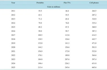
Table 2.Predicted sales amounts for portables computers, flat TVs, and cell phones.
Year Portables Flat TVs Cell phones
Units in millions
2011 55.5 46.4 264.5
2012 63.1 55.5 287.2
2013 71.2 65.4 310.9
2014 79.9 76.0 335.4
2015 89.2 87.5 360.9
2016 99.0 99.7 387.3
2017 109.5 112.8 414.5
2018 120.5 126.6 442.7
2019 132.0 141.2 471.8
2020 144.2 156.6 501.9
2021 156.9 172.8 532.8
2022 170.1 189.8 564.6
2023 184.0 207.6 597.4
2024 198.4 226.2 631.0
2025 213.4 245.6 665.6
referred to as the “second use” stage. There are many combinations of use, reuse, and storage underlying the
second use stage before the last user is ready for EOL management of the product. “Appendix Table C” shows the
assumed life span for the products and the percentage from the sales amount when the products reach their EOL.
3.3. Model Applied
In a socioeconomic system, products flow into the society (sales) and then accumulate in the built environment (stock); when reaching EOL after a certain period (life span), they flow out. The model presented in this study tries to estimate the future amount of e-waste in the United States. The model is a material flow analysis model, which is widely used to estimate the amount of waste in current years or to predict the waste that will be gener-ated in the future. The model inputs are the annual product sales data, historical sales data, and future sales data, which are predicted using the sales rate for the items whose sales are decreasing annually and polynomial re-gression analysis for the items whose annual sales are increasing.
In material flow analysis, the general form used to represent the outflow after the useful life span is a function of the inflow in the past and can be expressed by Equation (3).
outflow inflow
i
P
=
∑
× (3)where the outflow represents the waste generated and the inflow represent the sales amount and (P) is the
per-centage amount when the product reaches its end of life. Equations (4) and (5) show how the generated e-waste amount for desktops and portable computers are calculated.
( )
(
7)
(
)
(
9)
(
)
(
12)
(
)
(
15)
(
)
7,9,12,15
25% 25% 25% 25%
n n n n n
DC i
W S − S− S − S−
=
=
∑
× + × + × + × (4)where,
( )DCn
W =The amount of EOL generated from desktop computer products in year (n). S = historical and future
( )
(
3)
(
)
(
5)
(
)
(
6)
(
)
(
7)
(
)
3,5,6,720% 20% 30% 30%
n n n n n
PC i
W S− S− S− S−
=
=
∑
× + × + × + × (5)where,
( )PCn
W =The amount of EOL collected from portable computer products in year (n). S = historical and future
sales amount for portable computers product.
The amount collected for EOL management for CRT TVs product estimated by Equation (6).
( )
(
8)
(
)
(
11)
(
)
(
15)
(
)
(
17)
(
)
8,11,15,17
25% 25% 25% 25%
n n n n n
CTV i
W S− S− S− S−
=
=
∑
× + × + × + × (6)where,
(CTV)n
W = The amount collected for EOL management from CRT TV products in year (n). S = historical and
future sales amount for PC flat panel monitors.
Equation (7) for CRT PC monitor products to calculate the quantity collected for EOL management.
( )
(
5)
(
)
(
8)
(
)
(
10)
(
)
(
13)
(
)
.5,8,10,13
25% 25% 25% 25%
n n n n n
CM i
W S − S− S− S−
=
=
∑
× + × + × + × (7)where,
(CM)n
W = The EOL amount for CRT PC monitor products in year (n). S = historical and future sales amount
for CRT PC monitors.
Equation (8) calculates the amount collected for EOL management from PC flat monitor products.
( )
(
9)
(
)
(
10)
(
)
(
10)
(
)
(
11)
(
)
.9,10,11
80% 10% 25% 10%
n n n n n
FM i
W S− S− S− S−
=
=
∑
× + × + × + × (8)where,
(FM)n
W = The EOL for PC flat monitor products in year (n). S = historical and future sales amount for PC flat
panel monitors.
The EOL amount generated from hard copy peripherals product calculated by Equation (9).
( )
(
4)
(
)
(
7)
(
)
(
10)
(
)
(
14)
(
)
4,7,10,14
25% 25% 25% 25%
n n n n n
HCP i
W S− S− S − S −
=
=
∑
× + × + × + × (9)where,
(HCP)n
W = The amount collected for EOL management from HCP in year (n). S = historical and future sales
amount for Hard Copy Peripherals
The EOL quantity results from using keyboard products estimated by Equation (10).
( )
(
4)
(
)
(
5)
(
)
4,5
90% 10%
n n n
K i
W S − S −
=
=
∑
× + × (10)where,
( )KBn
W = The amount collected for EOL management from key board products in year (n). S = historical and
future sales amount for keyboard products.
The EOL quantity results from using mice products estimated by Equation (11)
( )
(
4)
(
)
(
5)
(
)
4,5
90% 10%
n n n
M i
W S− S−
=
=
∑
× + × (11)where,
( )Mn
W = The amount collected for EOL management from mice products in year (n). S = historical and future
sales amount for keyboard products.
Equation (11) estimates the future EOL amount for projector and monochrome products.
( , )
(
8)
(
)
(
9)
(
)
(
10)
(
)
8,9,10
80% 10% 10%
n n n n
PR MON i
W S− S− S−
=
=
∑
× + × + × (12)where,
(PR MON, )n
W = The amount collected for EOL management from projections and monochrome in year (n). S =
historical and future sales amount for projections and monochrome.
( )
(
2)
(
)
(
5)
(
)
(
6)
( )
2,5,665% 30% 5%
n n n n
CP i
W S− S− S−
=
=
∑
× + × + × (13)where,
( )CPn
W = The amount collected for EOL management from cell phone devices in year (n). S = historical and
future sales amount for cell phones.
3.4. Model Uncertainty
The authors used the coefficient of determination to assess the predictive power of the model. The R2is
com-puted as shown in Equation (14). The coefficient of determination, denoted R2or r2and pronounced R-squared,
is a number that indicates how well data fit a statistical model. It is a statistic used in the context of a statistic model whose main purpose is either the prediction of future outcomes or the testing of hypotheses. On the basis of other related information, it provides a measure of how well observed outcomes are replicated by the model
as the proportion of total variation of outcomes explained by the model. R2is a statistic that will give some
in-formation about the goodness of fit of a model. In regression, the R2coefficient of determination is a statistical
measure of how well the regression line approximates the real data points. An R2of 1 indicates that the
regres-sion line perfectly fits the data. The authors collected observation data from the USEPA [15]. The observation
data is the total amount collected for EOL management from 1999 to 2007. Observation and predicted data can
be found in Table 3. Figure 4 shows the predicted result against the observation data from 1999 through 2007
with an R2value of 9.4.
Figure 4.Model uncertainties, observation data against the predicted result.
Table 3. Observation and predicted data used to calculate the R2 value.
Year
Observation data* Predicted data*
Units in millions
1999 159.0 142.9
2000 161.6 167.7
2001 193.6 197.5
2002 225.2 243.0
2003 273.8 275.4
2004 310.7 288.3
2005 342.1 304.3
2006 342.9 327.2
2007 372.7 352.5
*Total amount collect for EOL management for all products.
0.0 50.0 100.0 150.0 200.0 250.0 300.0 350.0 400.0
1998 1999 2000 2001 2002 2003 2004 2005 2006 2007 2008
U
n
it
s in
M
illio
n
s
Year
(
)
(
)
2 obser obser-mean
2 1
2 obser
1 1
ˆ
n
n
Y Y
R
Y Y
−
= −
−
∑
∑
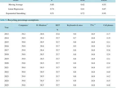
(14)3.5. Recycling and Disposed Amount
To estimate the portion of the recycled amount in the future three methods evaluated; moving average, linear re-gression and exponential smoothing, based on data from USEPA from 1999 through 2007, and to evaluate
which method is best among all, coefficient of determination (R2), mean absolute error (MAE) and root mean
square error (RMSE) performed, values can be found in Table 4. Based on the result for the above three
evolu-tion methods moving average found to be the best in terms of error forecasting and used to predict the
percen-tage of the recycling amount in the future as shown in Table 5 from total amount collected for EOL
manage-ment every year from 2013 through 2025, and the generated quantity that will be disposed calculated by sub-tracted the amount estimated to be recycled from the total estimated amount collected for EOL management.
3.6. Sensitivity Analysis
This study presents a sensitivity analysis for the model input, product life span, and predicted sales amount. It analyzes sensitivity analysis for product life span for three selected products: flat panel TVs, portable computers,
Table 4. R2, MAE and RMSE values for the moving average, linear regression and exponential smoothing methods used to
forecast the future recycling percentage.
Model R2 MAE RMSE
Moving Average 0.85 0.42 0.53
Linear Regression 0.74 0.61 0.67
[image:9.595.90.541.369.709.2]Exponential Smoothing 0.51 0.72 0.95
Table 5. Recycling percentage assmptions.
Year
Computers* Pc Monitors** HCP Keyboards & mice TVs*** Cell phones
%
2013 39.2 30.9 33.6 9.0 16.9 11.7
2014 38.9 30.2 33.7 8.7 16.8 11.9
2015 39.0 30.5 33.7 8.8 16.8 12.1
2016 39.0 30.6 33.7 8.9 16.8 12.4
2017 39.0 30.4 33.7 8.8 16.8 12.6
2018 39.0 30.5 33.7 8.8 16.8 12.9
2019 39.0 30.5 33.7 8.8 16.8 13.1
2020 39.0 30.5 33.7 8.8 16.8 13.4
2021 39.0 30.5 33.7 8.8 16.8 13.7
2022 39.0 30.5 33.7 8.8 16.8 14.0
2023 39.0 30.5 33.7 8.8 16.8 14.2
2024 39.0 30.5 33.7 8.8 16.8 14.5
2025 39.0 30.5 33.7 8.8 16.8 14.8
*
and cell phones. According to the literature review, the life span has great influence on the amount of generated waste. This analysis indicates the importance of the life span, the corresponding need for comprehensive know-ledge of consumer behavior, and the factors that affect the disposal decision such as technological innovation, availability, and cost of maintenance, among others. The idea is to increase the life span of those products by three years for portable computers and flat panel TVs, and two years for cell phones, and run the model to show how the generation of e-waste is affected by this change. The study presents a sensitivity analysis for product’s predicted sales amount to study the effect of the uncertainty of the predicted sales amount in the e-waste gener-ated quantity. The idea is to increase or decrease the prediction sales amount by 10%.
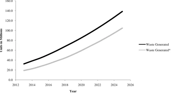
The results for products life span sensitivity analysis shows that the amount of waste will decrease as
pre-sented in Figures 5-7 and Tables 6-8.
Sensitivity analysis constructed for the predicted sales data in this study to evaluate the uncertainty of the
model. Assumed the predicted sales data will increase or decrease by 10%. Result shown in Tables 9-11,
in-dicted that the amount will be collected for EOL management will increase or decrease by the same amount of increasing in sales data in the future. Therefore the flow of the product in the market has a great influence in the waste amount as well as the accuracy of the sales data.
4. Results
[image:10.595.181.454.372.706.2]4.1. End of Life Management Amount
[image:10.595.174.455.375.530.2]Figure 8 shows the model result for amount collected for the EOL management from desktop computer prod-ucts. The result shows that the e-waste generated from this product is decreasing due to high increasing number of laptop user’s in recent years. The results indicated that about 15.6 million units could possible to be collected for end of life management in 2025.
Figure 5. Sensitivity analysis for portable computers life span.
Figure 6. Sensitivity analysis flat panel TVs life span.
0.0 20.0 40.0 60.0 80.0 100.0 120.0 140.0 160.0
2012 2014 2016 2018 2020 2022 2024 2026
U
n
it
s in
M
illio
n
s
Year
Waste Generated Waste Generated*
0.0 20.0 40.0 60.0 80.0 100.0 120.0
2012 2014 2016 2018 2020 2022 2024 2026
U
n
it
s in
M
illio
n
s
Year
[image:10.595.173.456.553.706.2]Figure 7. Sensitivity analyses for cell phones life span.
Figure 8. Desktop computer product end of the amount, model output.
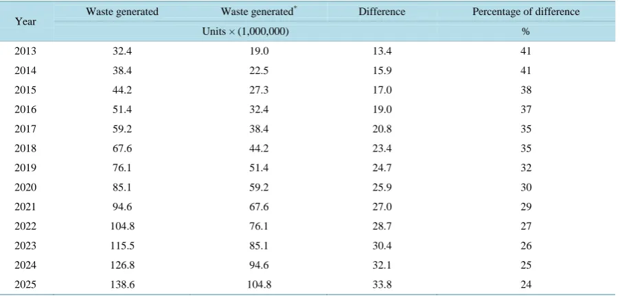
Table 6. Sensitivity analyses for portable computers life span.
Year Waste generated Waste generated
* Difference Percentage of difference
Units × (1,000,000) %
2013 32.4 19.0 13.4 41
2014 38.4 22.5 15.9 41
2015 44.2 27.3 17.0 38
2016 51.4 32.4 19.0 37
2017 59.2 38.4 20.8 35
2018 67.6 44.2 23.4 35
2019 76.1 51.4 24.7 32
2020 85.1 59.2 25.9 30
2021 94.6 67.6 27.0 29
2022 104.8 76.1 28.7 27
2023 115.5 85.1 30.4 26
2024 126.8 94.6 32.1 25
2025 138.6 104.8 33.8 24
*
Life span increased by 3 years.
The amount of products that can be collected for EOL management resulting from using portable computer
products will increase as per Figure 9. About 138.6 million units will reach their end of life in 2025. Compared
to the amount collected for EOL management estimated in this study in 2013, which is 34.2 million units, it is obvious that there will be a high increase in the collected amount of products for EOL management in the future.
0.00 100.00 200.00 300.00 400.00 500.00 600.00
2012 2014 2016 2018 2020 2022 2024 2026
U
n
it
s in
m
illio
n
s
Year
Waste Generated Waste Generated*
0.00 5.00 10.00 15.00 20.00 25.00 30.00 35.00 40.00
2013 2014 2015 2016 2017 2018 2019 2020 2021 2022 2023 2024 2025
U
n
it
s in
M
illio
n
Year
Table 7. Sensitivity analyses for flat panel TVs life span.
Year
Waste generated Waste generated* Difference Percentage
Units × (1,000,000) %
2013 32.4 19.0 13.4 41
2014 38.4 22.5 15.9 41
2015 44.2 27.3 17.0 38
2016 51.4 32.4 19.0 37
2017 59.2 38.4 20.8 35
2018 67.6 44.2 23.4 35
2019 76.1 51.4 24.7 32
2020 85.1 59.2 25.9 30
2021 94.6 67.6 27.0 29
2022 104.8 76.1 28.7 27
2023 115.5 85.1 30.4 26
2024 126.8 94.6 32.1 25
2025 138.6 104.8 33.8 24
*Life span increased by 3 years.
Table 8. Sensitivity analysis for cell phone life span.
Year
Waste generated Waste generated* Difference Percentage
Units × (1,000,000) %
2013 240.52 197.50 43.03 18
2014 261.46 215.97 45.49 17
2015 283.56 240.52 43.04 15
2016 309.17 261.46 47.71 15
2017 333.98 283.56 50.42 15
2018 359.35 309.17 50.18 14
2019 385.63 333.98 51.65 13
2020 412.82 359.35 53.47 13
2021 440.92 385.63 55.29 13
2022 469.93 412.82 57.11 12
2023 499.86 440.92 58.93 12
2024 530.69 469.93 60.75 11
2025 562.43 499.86 62.58 11
*
Life span increased by 2 years.
Hard copy peripherals (HCPs) include printers, multifunction printers, digital copiers, and faxes. Figure 10
shows the model result; 13.4 million units will be collected for EOL management in 2025.
The model estimated about 1.7 million units and 97.0 million units will reach their end of life from CRT and
[image:12.595.88.542.398.646.2]Table 9. Sensitivity analysis for predicted sales data for portable computers product.
Year
Model EOL (+%10)* (−%10)** % for (+%10) % for (−%10)
Units × (1,000,000) (%)
2013 32.39 32.39 32.39 0 0
2014 38.41 39.52 37.30 3 -3
2015 44.24 45.50 42.98 3 -3
2016 51.38 53.91 48.84 5 -5
2017 59.16 63.68 54.64 8 -8
2018 67.64 74.41 60.88 10 -10
2019 76.07 83.67 68.46 10 -10
2020 85.06 93.57 76.56 10 -10
2021 94.63 104.09 85.17 10 -10
2022 104.77 115.25 94.29 10 -10
2023 115.48 127.02 103.93 10 -10
2024 126.76 139.43 114.08 10 -10
2025 138.60 152.47 124.74 10 -10
(+%10)*= 10% increasing in prediction sales quantity, (−%10) **= 10% decreasing in prediction sales quantity.
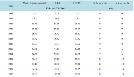
Table 10. Sensitivity analysis for predicted sale data for flat panel TVs product.
Year
Model E-waste Amount (+%10)* (−%10)**
% for (+%10) % for (−%10)
Units ×(1,000,000) (%)
2013 2.28 2.28 2.28 0 0
2014 4.93 4.93 4.93 0 0
2015 11.56 11.56 11.56 0 0
2016 18.15 18.15 18.15 0 0
2017 26.62 26.62 26.62 0 0
2018 30.62 30.62 30.62 0 0
2019 33.07 33.07 33.07 0 0
2020 43.88 47.61 40.15 9 -9
2021 52.68 57.61 47.75 9 -9
2022 62.89 69.18 56.60 10 -10
2023 73.46 80.80 66.11 10 -10
2024 84.84 93.32 76.35 10 -10
2025 97.03 106.73 87.32 10 -10
(+%10)*= 10% increasing in prediction sales quantity, (−%10) **= 10% decreasing in prediction sales quantity.
Computer accessory in this study refer to keyboards and mice. Keyboards model result shown in Figure 12
and mice in Figure 13. The predicted amount collected for EOL management from these two products in 2025
Table 11. Sensitivity analyses for predicted sales data for cell phone product.
Year
Model E-waste Amount (+%10)* (−%10)** % for (+%10) % for (−%10)
Units × (1,000,000) (%)
2013 240.52 257.72 223.33 7 -7
2014 261.46 280.13 242.79 7 -7
2015 283.56 303.77 263.35 7 -7
2016 309.17 338.91 279.43 10 -10
2017 333.98 367.38 300.59 10 -10
2018 359.35 395.29 323.42 10 -10
2019 385.63 424.20 347.07 10 -10
2020 412.82 454.10 371.54 10 -10
2021 440.92 485.02 396.83 10 -10
2022 469.93 516.93 422.94 10 -10
2023 499.86 549.84 449.87 10 -10
2024 530.69 583.76 477.62 10 -10
2025 562.43 618.67 506.19 10 -10
(+%10)*= 10% increasing in prediction sales quantity, (−%10) **= 10% decreasing in prediction sales quantity.
Figure 9. Portable computer end of life amount, model output.
Figure 10. Hard copy peripherals end of life amount, model output.
0.00 20.00 40.00 60.00 80.00 100.00 120.00 140.00 160.00
2013 2014 2015 2016 2017 2018 2019 2020 2021 2022 2023 2024 2025
U
n
it
s in
M
illio
n
s
Year
Portable Computers
0.00 5.00 10.00 15.00 20.00 25.00 30.00 35.00
2013 2014 2015 2016 2017 2018 2019 2020 2021 2022 2023 2024 2025
U
n
it
s in
M
illio
n
s
Year
[image:14.595.167.468.562.703.2]Figure 11. CRT and flat panel monitors end of life amount, model output.
Figure 12. Keyboards end of life amount, model output.
Figure 13. Mice end of life amount, model output.
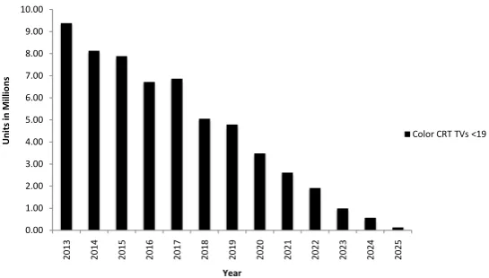
Color CRT TV < 19 inches product quantity will be collected for EOL management in 2025 is 0.13 million
units as per the model result as presented in Figure 14. The future EOL amount for color CRT TV > 19 inch
products estimated about 0.26 million, Figure 15 shows the result from 2013 to 2025.
Figure 16 illustrated the forecasted amount collected for EOL management from 2013 through 2025 for flat panel TV products. The collected quantity in 2025 is 97.0 million units.
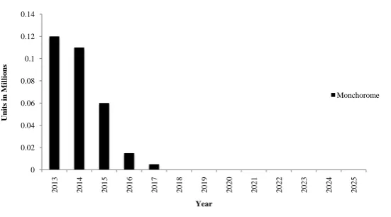
Figure 17 shows the prediction e-waste amount for projectors, about 0.11 million units reach their end of life in 2025.
Prediction waste amount for monochrome, in 2013 is about 0.12 million units and will be zero from 2018 as
shown in Figure 18.
The e-waste amount for cell phones shows in Figure 19. The model estimates that the amount will be col-
0.00 5.00 10.00 15.00 20.00 25.00 30.00 35.00 40.00
2013 2014 2015 2016 2017 2018 2019 2020 2021 2022 2023 2024 2025
U
n
it
s in
M
ilio
n
s
Year
CRT Monitors
Flat Panel Monitors
0.00 5.00 10.00 15.00 20.00 25.00 30.00 35.00 40.00
2013 2014 2015 2016 2017 2018 2019 2020 2021 2022 2023 2024 2025
U
n
it
s in
M
illo
n
s
Year
keyboards
0.00 5.00 10.00 15.00 20.00 25.00
2013 2014 2015 2016 2017 2018 2019 2020 2021 2022 2023 2024 2025
U
n
it
s in
M
illio
n
s
Year
Figure 14. Color CRT TVs < 19 inches end of life amount, model output.
Figure 15. Color CRT TVs > 19 inches end of life amount, model output.
Figure 16. Flat panel TVs end of life amount, model output.
lected for EOL management is about 562.4.82 million units in 2025.
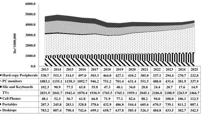
4.2. Generation Waste Amount by Weight
This section presents estimates of the quantity of EOL management for electronic and electrical products gener-ated for management each year by weight. As described earlier, we developed the estimates by starting with product sales data and assuming specific life spans for each product type to represent the time between product purchase and the need for EOL management. The average weight of products is an important factor in the amount of the e-waste generation. Within some product types, such as TVs, weights vary depending on the size
and type of screen. Product weights also can vary over time as technology, style, and features change [15]. The
0.00 1.00 2.00 3.00 4.00 5.00 6.00 7.00 8.00 9.00 10.00
2013 2014 2015 2016 2017 2018 2019 2020 2021 2022 2023 2024 2025
U
nit
s in
M
illio
ns
Year
Color CRT TVs <19 inch
0.00 5.00 10.00 15.00 20.00
2013 2014 2015 2016 2017 2018 2019 2020 2021 2022 2023 2024 2025
U
n
it
s in
M
illio
n
s
Year
Color CRT TVs >19 inch
0.00 20.00 40.00 60.00 80.00 100.00 120.00
2013 2014 2015 2016 2017 2018 2019 2020 2021 2022 2023 2024 2025
U
n
it
s in
M
illio
n
s
Year Flat Panel TVs
[image:16.595.173.446.83.238.2] [image:16.595.174.456.263.408.2]Figure 17. Projectors end of life amount, model output.
Figure 18. Monochrome end of life amount, model output.
weight of the products is adopted from [14] [15]. Tables 12-14 and Figures 20-22 presented total quantity
col-lected for EOL management for all products. Tables 15 shows the percentage of each product collected for EOL
management by units from the total amount collected for EOL management, while Table 16shows the
percen-tage of every product collected for EOL management by weight. The cell phone product is the highest among the all products which will be collected for EOL management by units and the lowest by weight.
4.3. Recycling and Disposed Amount
The majority of EOL material that is not being recycled is probably going into landfills, about 80% from the to-tal EOL amount will go to landfills in 2025. Refer to, “even though cell phone devices are the highest product estimated in this study will be recycled still is the highest product will be land filled” followed by computers, TVs, Keyboards, mice, PC monitors and hard copy peripherals.
According to this analysis about 60.1 million units of computer products, 16.6 million units of TVs 83.3 million units from cell phones, 4.3 million units of computer displayers, 0.7 million units of keyboards and mice and 4.5
from hard copy peripherals will be recycled in 2025 as shown in “Table 17” and “Figure 21”. The amount will be
disposed shown in “Table 18” and “Figure 23”. The total amount will be recycled is about 30% from the total
amount collected for EOL management in 2025.
5. Conclusions and Discussion
The purpose of this study was to establish a baseline regarding the management of EOL electrical and electronic products (e-waste). The baseline data addresses televisions, cell phones, personal computers (desktops, laptops), computer displayers (CRT and flat monitors), keyboards, mice, and hard copy devices (e.g., printers, scanners, faxes) are sold between 1980 and 2025.
The quantity collected for EOL management from desktop computer products will decrease; 35.9 million units are predicted to reach their EOL in 2015 and 15.6 million units in 2025.
The collected EOL amount for portable computer products is 44.2 million units in 2015 and about 138.6 mil
0.0000 0.5000 1.0000 1.5000 2.0000 2.5000 3.0000 3.5000
2013 2014 2015 2016 2017 2018 2019 2020 2021 2022 2023 2024 2025
U
n
it
s in
M
illio
n
s
Year
Color Projectrs
0 0.02 0.04 0.06 0.08 0.1 0.12 0.14
2013 2014 2015 2016 2017 2018 2019 2020 2021 2022 2023 2024 2025
U
n
it
s in
M
illio
n
s
Year
[image:17.595.179.455.239.392.2]Figure 19. Cell phones end of life amount, model output.
Figure 20. Waste generations amount by weight.
Figure 21. Waste generations amount by units.
lion units in 2025. This study shows that there will be more portable computers in the market than desktop
computers in the future [16]. Therefore, there will be more e-waste generated from portable computers. We es-
0.0 100.0 200.0 300.0 400.0 500.0 600.0
2013 2014 2015 2016 2017 2018 2019 2020 2021 2022 2023 2024 2025
U
n
it
s in
m
illio
n
s
Year
Cell phones
2013 2014 2015 2016 2017 2018 2019 2020 2021 2022 2023 2024 2025 Hard copy Peripherals 530.7 553.3 514.5 497.0 503.3 464.0 427.1 410.2 385.0 337.1 294.4 270.7 232.8 PC monitors 1083.1 1155.1 1158.3 1092.7 946.2 751.2 701.4 631.4 551.5 488.0 431.6 381.9 337.9 Mic and Keyboards 102.3 90.9 77.5 65.8 55.8 47.3 40.1 34.0 28.8 24.4 20.7 17.6 14.9 TVs 2031.9 2041.7 1942.4 1870.4 1936.9 1765.5 1765.1 1959.1 2045.1 2106.8 2188.9 2263.9 2466.7 Cell Phones 48.1 52.3 56.7 61.8 66.8 71.9 77.1 82.6 88.2 94.0 100.0 106.1 112.5 Portables 207.3 245.8 283.1 328.8 378.6 432.9 486.8 544.4 605.6 670.5 739.1 811.2 887.1 Desktops 783.2 807.4 790.4 742.6 699.1 658.7 637.8 585.4 526.3 484.8 433.5 382.7 342.5
0.0 1000.0 2000.0 3000.0 4000.0 5000.0 6000.0
lb
s*1000,
000
2013 2014 2015 2016 2017 2018 2019 2020 2021 2022 2023 2024 2025
Hard copy Peripherals 30.5 31.8 29.6 28.6 28.9 26.7 24.5 23.6 22.1 19.4 16.9 15.6 13.4
PC monitors 32.3 38.5 41.6 40.5 36.0 29.6 28.2 25.3 22.4 19.8 17.5 15.5 13.7
Mic and Keyboards 57.4 50.2 42.8 36.3 30.8 26.1 22.1 18.8 15.9 13.5 11.4 9.7 8.2
TVs 30.8 32.2 36.1 39.7 46.6 46.9 48.8 58.3 64.8 72.5 80.0 88.3 98.8
Cell Phones 240.5 261.5 283.6 309.2 334.0 359.4 385.6 412.8 440.9 469.9 499.9 530.7 562.4
Portables 32.4 38.4 44.2 51.4 59.2 67.6 76.1 85.1 94.6 104.8 115.5 126.8 138.6
Desktops 35.6 36.7 35.9 33.8 31.8 29.9 29.0 26.6 23.9 22.0 19.7 17.4 15.6
0.0 100.0 200.0 300.0 400.0 500.0 600.0 700.0 800.0 900.0
U
n
it
s in
M
illio
n
[image:18.595.145.484.485.687.2]Figure 22. Recycling generation amount by units.
Figure 23.Disposed generation amount by units.
timate that computer products (desktops and portables) will be one of the most commonly recycled products in the future with about 7% of the total quantity collected for EOL management, and the quantity that will be dis-posed is about 11%, unless there is a ban on dumping them in landfills.
For hard copy peripheral products, the study estimated about 13.4 million units will reach their EOL in 2025. Respectively, 4.5 million units and 8.9 million units will be recycled and disposed.
The amount collected for EOL management forecasted by the model for computer displayers is about 0.0 and 13.34 million units for CRT and flat panel monitor products, respectively, in 2025. Over the last five to seven
years, flat panel monitors have taken over as the predominant monitors to be used with a computer [17]. Of
these, 4.3 million units are estimated to be recycled and about 9.4 million units will be disposed.
Computer accessories in this study refer to keyboards and mice. The model result estimated about 4.9 and 3.3 million units will reach their EOL in 2025 for keyboard and mouse products, respectively. The recycled amount is less than the disposed amount; 7.5 million units will be disposed and 0.7 million units will be recycled for both products.
This study carried out predictions of EOL amounts for three types of TVs: color CRT TVs greater and less than 19 inches and flat panel TVs. The predicted sales amount estimated in this study shows that the CRT TV sales will reach 0.00 in 2016. However, the amount of e-waste generated from these two products is considera-
2013 2014 2015 2016 2017 2018 2019 2020 2021 2022 2023 2024 2025
HCP 10.2 10.7 10.0 9.6 9.7 9.0 8.3 7.9 7.4 6.5 5.7 5.2 4.5
Keyboards & Mice 5.2 4.4 3.8 3.2 2.7 2.3 2.0 1.7 1.4 1.2 1.0 0.9 0.7
Pc monitors 10.2 12.2 13.2 12.8 11.4 9.4 8.9 8.0 7.1 6.3 5.6 4.9 4.3
Cell phones 28.1 31.1 34.4 38.3 42.2 46.3 50.7 55.4 60.3 65.6 71.1 77.0 83.3
TVs 5.2 5.4 6.1 6.7 7.8 7.9 8.2 9.8 10.9 12.2 13.5 14.9 16.6
Computers 26.6 29.2 31.3 33.2 35.4 38.1 41.0 43.5 46.2 49.5 52.7 56.2 60.1
0.0 20.0 40.0 60.0 80.0 100.0 120.0 140.0 160.0 180.0
U
n
it
s in
M
illio
n
s
2013 2014 2015 2016 2017 2018 2019 2020 2021 2022 2023 2024 2025
HCP 20.3 21.1 19.6 19.0 19.2 17.7 16.3 15.6 14.7 12.8 11.2 10.3 8.9
Keyboards & Mice 52.2 45.9 39.0 33.0 28.0 23.8 20.2 17.1 14.5 12.3 10.4 8.8 7.5
Pc monitors 22.1 26.3 28.5 27.7 24.6 20.2 19.3 17.3 15.3 13.6 12.0 10.6 9.4
Cell phones 212.4 230.3 249.1 270.9 291.8 313.0 334.9 357.5 380.6 404.4 428.7 453.7 479.2
TVs 25.6 26.8 30.0 33.0 38.8 39.0 40.6 48.5 53.9 60.3 66.5 73.4 82.1
Computers 41.3 45.9 48.9 51.9 55.5 59.5 64.1 68.1 72.3 77.3 82.5 87.9 94.0
0.0 100.0 200.0 300.0 400.0 500.0 600.0 700.0 800.0
U
n
it
s in
M
illio
n
Table 12. Desktops and portables computer amount collected for EOL management by weight.
Year
Desktops Portables Cell phones
Units × (1,000,000)
Weight (lbs) × (1,000,000)
Units × (1,000,000)
Weight (lbs) × (1,000,000)
Units × (1,000,000)
Weight (lbs) × (1,000,000)
2013 35.6 783.2 32.4 207.3 240.5 48.1
2014 36.7 807.4 38.4 245.8 261.5 52.3
2015 35.9 790.4 44.2 283.1 283.6 56.7
2016 33.8 742.6 51.4 328.8 309.2 61.8
2017 31.8 699.1 59.2 378.6 334.0 66.8
2018 29.9 658.7 67.6 432.9 359.4 71.9
2019 29.0 637.8 76.1 486.8 385.6 77.1
2020 26.6 585.4 85.1 544.4 412.8 82.6
2021 23.9 526.3 94.6 605.6 440.9 88.2
2022 22.0 484.8 104.8 670.5 469.9 94.0
2023 19.7 433.5 115.5 739.1 499.9 100.0
2024 17.4 382.7 126.8 811.2 530.7 106.1
2025 15.6 342.5 138.6 887.1 562.4 112.5
Table 13. Color CRT TVs and flat panel TVs amount collected for EOL management by weight.
Year
Color CRT < 19 inch Color CRT > 19 inch Flat panel TVs
Units × (1,000,000)
Weight (lbs) × (1,000,000)
Units × (1,000,000)
Weight (lbs) × (1,000,000)
Units × (1,000,000)
Weight (lbs) × (1,000,000)
2013 9.60 393.6 15.82 1154.5 2.28 56.1
2014 8.61 353.1 15.41 1124.6 4.93 121.3
2015 8.73 358.0 13.54 988.2 11.56 284.4
2016 7.52 308.3 12.65 923.8 18.15 446.5
2017 7.22 295.9 11.95 872.7 26.62 654.8
2018 6.39 261.9 9.57 698.6 30.62 753.2
2019 6.61 270.8 8.94 652.5 33.07 813.5
2020 5.67 232.6 8.66 632.4 43.88 1079.4
2021 4.30 176.3 7.85 572.8 52.68 1295.9
2022 4.32 177.1 5.24 382.6 62.89 1547.1
2023 2.95 120.8 3.57 261.0 73.46 1807.1
2024 2.28 93.7 1.14 83.3 84.84 2087.0
2025 1.49 61.1 0.26 18.7 97.03 2386.9
ble because of the assumption of the life span and their weight. The study predicts that 0.13 million units will be collected for EOL management from color TVs < 19 inches and 0.26 million units from color TVs > 19 inches in 2025.
Table 14. Projections, flat panel PC monitors amount collected for EOL management by weight.
Year
Projections Flat Panel Monitors CRT Monitors
Units × (1,000,000)
Weight (lbs) × (1,000,000)
Units × (1,000,000)
Weight (lbs) × (1,000,000)
Units × (1,000,000)
Weight (lbs) × (1,000,000)
2013 3.0 422.8 21.13 519.8 11.15 563.3
2014 3.1 438.2 30.47 749.6 8.03 405.5
2015 2.2 309.4 36.45 896.7 5.18 261.6
2016 1.4 191.2 36.76 904.3 3.73 188.4
2017 0.8 113.3 33.72 829.5 2.31 116.7
2018 0.4 51.9 28.73 706.8 0.88 44.4
2019 0.2 28.4 27.99 688.6 0.25 12.9
2020 0.1 14.7 24.94 613.4 0.36 18.0
2021 0.0 0.1 22.41 551.2 0.00 0.2
2022 0.0 0.0 19.83 487.8 0.00 0.2
2023 0.0 0.0 17.54 431.6 0.00 0.0
2024 0.0 0.0 15.52 381.9 0.00 0.0
2025 0.0 0.0 13.74 337.9 0.00 0.0
Table 15. Estimated for EOL Management percentage (%) of total per units.
Year
Desktops Portables Cell Phones CRT TVs Flat TVs Projections & Monochrome
Mice and
Keyboards PC Monitors Total
Estimated for EOL Management Percentage of Total (%) per Units
2013 8 8 56 6 1 1 13 8 100
2014 8 8 57 5 1 1 11 8 100
2015 7 9 59 5 2 0 9 9 100
2016 7 10 61 4 4 0 7 8 100
2017 6 11 62 4 5 0 6 7 100
2018 5 12 64 3 5 0 5 5 100
2019 5 13 65 3 6 0 4 5 100
2020 4 14 66 2 7 0 3 4 100
2021 4 14 67 2 8 0 2 3 100
2022 3 15 67 1 9 0 2 3 100
2023 3 16 67 1 10 0 2 2 100
2024 2 16 67 0 11 0 1 2 100
2025 2 17 67 0 12 0 1 2 100
the total collected amount for EOL management, and 10% will be disposed in 2025.
[image:21.595.91.537.384.647.2]Table 16. Estimated EOL Management percentage of total (%) per weight.
Year
Desktops Portables Cell Phones CRT TVs Flat TVs Projections & Monochrome
Mice and
Keyboards PC Monitors Total
Estimated for EOL Management percentage of total (%) per weight
2013 18 5 1 36 1 10 2 25 100
2014 18 6 1 34 3 10 2 26 100
2015 18 7 1 31 7 7 2 27 100
2016 18 8 1 30 11 5 2 26 100
2017 17 9 2 29 16 3 1 23 100
2018 18 12 2 26 20 1 1 20 100
2019 17 13 2 25 22 1 1 19 100
2020 15 14 2 23 28 0 1 16 100
2021 14 16 2 19 34 0 1 14 100
2022 13 17 2 14 40 0 1 13 100
2023 11 19 3 10 46 0 1 11 100
2024 10 20 3 4 53 0 0 10 100
2025 8 21 3 2 57 0 0 8 100
Table 17. Recycling generation amount by units.
Year
Computers* PC
Monitors** HCP Keyboards & Mice TVs***
Units × (1,000,000)
2013 26.6 5.2 28.1 10.2 5.2
2014 29.2 5.4 31.1 12.2 4.4
2015 31.3 6.1 34.4 13.2 3.8
2016 33.2 6.7 38.3 12.8 3.2
2017 35.4 7.8 42.2 11.4 2.7
2018 38.1 7.9 46.3 9.4 2.3
2019 41.0 8.2 50.7 8.9 2.0
2020 43.5 9.8 55.4 8.0 1.7
2021 46.2 10.9 60.3 7.1 1.4
2022 49.5 12.2 65.6 6.3 1.2
2023 52.7 13.5 71.1 5.6 1.0
2024 56.2 14.9 77.0 4.9 0.9
2025 60.1 16.6 83.3 4.3 0.7
*Desktops & portable computers, **CRT & flat monitors, ***CRT TVs, flat TVs, projections and monochrome.
units will be disposed. The product is the most common to be recycled but also the most common to be disposed, and the recycling is weighed at about 10% from the total amount collected for EOL management in 2025 by units.
[image:22.595.95.539.380.644.2]Table 18. Disposed generation amount by units.
Year
Computers* PC Monitors** HCP Keyboards & Mice TVs***
Units × (1,000,000)
2013 41.3 25.6 212.4 22.1 52.2
2014 45.9 26.8 230.3 26.3 45.9
2015 48.9 30.0 249.1 28.5 39.0
2016 51.9 33.0 270.9 27.7 33.0
2017 55.5 38.8 291.8 24.6 28.0
2018 59.5 39.0 313.0 20.2 23.8
2019 64.1 40.6 334.9 19.3 20.2
2020 68.1 48.5 357.5 17.3 17.1
2021 72.3 53.9 380.6 15.3 14.5
2022 77.3 60.3 404.4 13.6 12.3
2023 82.5 66.5 428.7 12.0 10.4
2024 87.9 73.4 453.7 10.6 8.8
2025 94.0 82.1 479.2 9.4 7.5
*Desktops & portable computers, **CRT & flat monitors, ***CRT TVs, flat TVs, projections and monochrome.
ucts. The disposal amount weighed about 80.0% from the total amount collected for EOL management
com-pared to the result of a USEPA report for 2008 [4], which stated that about 80.1%. The result shows no change
in the amount will go to the landfills in future and means that all the states authorities need to establish appropriate infrastructures and regulations to increase the recycling amount.
Sensitivity analysis shows that the product life span has an effect on the quantity of the e-waste that will be generated from the products under study. For example, e-waste will decrease about 20% if the life span for portable computer products increases by three years in 2025, while the sensitivity analysis for forecasted future sales indicates that the generated waste will increase or decrease according to the sales trend.
The e-waste amount per capita is estimated to be about 12.71 lbs./cap in 2025 compared to the result of a USEPA 2009 report, which shows 6.34 lbs./cap. This indicts that e-waste amount per capita in 2025 will be two
times the estimated amount by USEPA in 2009 [4].
This study is based on data collected from the USEPA, assumptions for products’ life span, and the percen-tage of products ready for EOL based on data from State of Florida and is assumed to be representative for all other states. This assumption may misrepresent product usage patterns, which could have an effect on the quan-tity collected for EOL management.
Acknowledgements
This work was sponsored by the Department of Energy Samuel Massie Chair of Excellence Program under Grant No. DE-NA0000718. The views and conclusions contained herein are those of the writers and should not be interpreted as necessarily representing the official policies or endorsements, either expressed or implied, of the funding agency.
References
[1] Dwivedy, M. and Mittal, R.K. (2010) Estimation of Future Outflows of E-Waste in India. Waste Management, 30, 483-
491. http://dx.doi.org/10.1016/j.wasman.2009.09.024
[2] Kang, H.Y. and Schoenung, J. M. (2006) Estimation of Future Outflows and Infrastructure Needed to Recycle Personal
http://dx.doi.org/10.1016/j.jhazmat.2006.03.062
[3] Gustavo, R., Flávia, G., Martin, S., Susane, P., Renato, A. and Ribeiro, C. (2009) Diagnosis of Waste Electric and
Electronic Equipment Generation in the State of Minas Gerais. Swiss Federal Laboratories for Materials Science and Technology (EMPA). (In Portuguese)
[4] United States Environmental Protection Agency (2011) Electronics Waste Management in the United States through
2009. http://www.epa.gov
[5] Steubing, B., Boni, H., Schluep, M., Silva, U. and Ludwig, C. (2010) Assessing Computer Waste Generation in Chile
Using Material Flow Analysis. Waste Management, 30, 473-482. http://dx.doi.org/10.1016/j.wasman.2009.09.007
[6] Ibrahim, F.B., Adie, D.B., Giwa, A.R., Abdullahi, S.A. and Okuofu, C.A. (2013) Material Flow Analysis of Electronic
Wastes (E-Wastes) in Lagos, Nigeria. Journal of Environmental Protection, 4, 1011-1017. http://dx.doi.org/10.4236/jep.2013.49117
[7] Araujo, M.G., Magrini, A., Mahler, C.F. and Bilitewski, B. (2012) A Model for Estimation of Potential Generation of
Waste Electrical and Electronic Equipment in Brazil. Waste Management, 32, 335-342. http://dx.doi.org/10.1016/j.wasman.2011.09.020
[8] Oguchi, M., Kameya, T., Yagi, S. and Urano, K. (2008) Product Flow Analysis of Various Consumer Durables in
Ja-pan. Resources, Conservation and Recycling, 52, 463-480. http://dx.doi.org/10.1016/j.resconrec.2007.06.001
[9] Voet, E., Kleijn, R., Huele, R., Ishikawa, M. and Verkuijlen, E. (2002) Special Section: European Environmental
His-tory and Ecological Economics. Ecological Economics, 41, 223-234.
[10] Lau, W.K., Chung, S.S. and Zhang, C. (2013) A Material Flow Analysis on Current Electrical and Electronic Waste
Disposal from Hong Kong households. Waste Management, 33, 714-721. http://dx.doi.org/10.1016/j.wasman.2012.09.007
[11] Liu, X., Tanaka, M. and Matsui, Y. (2006) Generation Amount Prediction and Material Flow Analysis of Electronic
Waste: A Case Study in Beijing, China. Waste Management and Research, 24, 434-435.
[12] Kahhat, R. and Williams, E. (2012) Materials Flow Analysis of E-Waste: Domestic Flows and Exports of Used
Com-puters from the United States. Resources, Conservation and Recycling, 67, 67-74. http://dx.doi.org/10.1016/j.resconrec.2012.07.008
[13] Morias, J.M., Van Liew, M.W., Binger, R.L., Harmel, R.D. and Veith, T.L. (2007) Model Evaluation Guidance for
Systematic Qualification of Accuracy in Watershed Simulation. American Society of Agricultural and Biological
En-gineering, 50, 885-900.
[14] United States Protection Agency (U.S.EPA) (2007) Management of Electronic Waste in the United States: Approach
Two. http://www.epa.gov
[15] United States Protection Agency (USEPA) (2008) Electronic Waste Management in United States: Approach 1.
http://www.epa.gov
[16] Statista (2015) Number of Smartphone Users in the US from 2010 to 2018 (in millions). http://www.statista.com
Appendix
Table A1. Historical sales data for computers, HCP, computer accessories and computer displayer.
Year
Computers Computer Peripherals & Accessories Computer Displays
Desktops Portables Hard Copy Peripherals Mice Keyboards PC CRTs PC Flat Panel
Units × (1,000,000)
1980 1.0 0.0 5.0 1.0 1.0 1.0 0.0
1981 2.0 0.0 1.0 2.0 2.0 2.0 0.0
1982 3.0 0.0 1.6 3.0 3.0 3.0 0.0
1983 5.5 0.0 2.9 5.5 5.5 5.5 0.0
1984 6.7 0.0 3.5 6.7 6.7 6.7 0.0
1985 5.8 0.0 3.0 5.8 5.8 5.8 0.0
1986 6.9 0.0 3.6 6.9 6.9 6.9 0.0
1987 8.2 0.0 4.3 8.2 8.2 8.2 0.0
1988 8.7 0.0 4.6 8.7 8.7 8.7 0.0
1989 8.9 0.0 4.7 8.9 17.5 8.4 1.1
1990 9.5 0.0 5.0 9.5 21.7 9.4 0.9
1991 9.5 0.0 5.0 9.5 27.0 10.5 1.5
1992 9.9 1.9 6.2 9.9 37.6 13.4 1.7
1993 13.0 2.5 8.2 13.0 36.1 17.3 1.8
1994 15.3 3.2 9.7 15.3 41.4 18.1 2.8
1995 19.1 3.6 11.9 19.1 47.6 22.2 3.0
1996 22.4 4.9 14.9 22.4 53.8 23.1 2.3
1997 26.8 6.0 16.2 26.8 55.6 26.6 0.9
1998 32.5 6.4 22.5 32.5 65.0 32.6 1.5
1999 39.5 7.9 27.5 39.5 63.7 36.9 2.8
2000 40.8 9.6 28.7 40.8 51.7 37.5 4.8
2001 35.1 9.6 26.8 35.1 43.8 27.2 6.6
2002 35.1 10.9 28.7 35.1 48.6 23.3 11.7
2003 37.0 13.8 30.7 37.0 51.3 15.8 18.0
2004 39.4 16.6 32.2 39.4 47.2 13.9 22.7
2005 38.0 19.6 33.1 41.2 44.1 7.8 33.0
2006 35.4 24.3 34.3 35.4 44.6 3.5 38.6
2007 34.2 30.0 36.9 34.2 43.1 1.0 37.0
2008 30.5 34.1 33.1 30.5 38.4 1.4 32.7
2009 26.3 40.4 29.5 26.3 33.1 0.0 27.2
2010 23.5 46.4 29.4 23.5 29.6 0.0 27.5