Time Series Prediction using Multiwavelet Transform
and Echo State Network
ABSTRACT
The accuracy of forecasts is influenced by both the quality of past data and the method selected to forecast the future. This paper shows a method to accurately predict the time series signal through a combination of decomposition methods and Echo State Network (ESN). Wavelet and Multiwavelet transforms are used to decompose highly nonlinear time series into several stationary time series components. Thereby, they are used to reduce the degree of nonlinear time series and make the issue easy to analyze and predict. These components are fed to an ESN, which predicts the signal. As an illustration for proposed pattern, one of time series signals of the neural network competition (NNC 2010) is used, without knowing its properties. The performances of all the methods used in this work have been evaluated by computer using MATLAB 7.9.0.287 (R2009b) language and RCToolbox version 2.1. Finally, comparison between these two transforms was done in terms of mean square error (MSE). The simulation results showed the effectiveness and significant improvement of the MWT-ESN model compared with DWT-ESN.
General Terms
Time Series Prediction ,Echo State Network ,Forcasting
Keywords
Discrete Wavelet Transform, Discrete Multiwavelet Transform, Recurrent Neural Network, Reservoir Computing, Echo State Network.
1.
INTRODUCTION
Time series prediction is the procedure of forecasting of measurements based on the trends of the past values measured in uniform interval [1]. The ability to make a good prediction of the future is advantageous in a broad range of applications. Companies and government organizations use medium- to short-term predictions for planning and operation of their businesses.
A large number of researchers are working on time series prediction, because of the great interest in time series prediction. These researchers come from a wide variety of fields and try to model the underlying process using linear techniques such as [1] and exponential smoothing [2] or non-linear techniques such as ARMA (Auto-regressive Moving Average) models [1]and neural networks [3]. They found that decomposition of time series process increased theaccuracy of forecasts, which is the main aim of the forecasting process [4].
The domain of time series prediction using neural network techniques was increased [5]. In last years, an important number of works related to the use of recurrent neural networks (RNNs) for time series prediction have been published. Recurrent neural networks are gaining success because they are ideal for such a temporal task. This kind of networks has an internal feedback loop which gives them the ability to model temporal relationship of the time series explicitly within their internal states [6]. Unfortunately, these networks suffers from complexity in training even with the existence of good training algorithms, The RNNs technique in nonlinear modeling has remained limited for a long time. The main reason for this lies in the fact that RNNs are difficult to train by descent based methods ), which aim iteratively to reduce training error. Reservoir computing is a novel technique for the fast training of large recurrent neural networks which have been successfully applied in a broad range of temporal tasks such as robotics [7], [8], speech recognition and time series generation. The reservoir computing technique is based on the use of a large untrained dynamical system, the reservoir, where the desired function is implemented by a linear memory-less mapping from the full instantaneous state of the dynamic system to the desired output. Only this linear mapping is learned. When the dynamical system is a recurrent neural network of analog neurons the method is referred to as echo state networks [7]. When spiking neurons are used, the method is referred to as liquid state machines [8]. But both are now commonly referred to as reservoir computing [9]. The main advantages of reservoir computing are its elegance and simplicity of use. When solving an offline problem using reservoirs, one constructs a random network with a certain topology, simulates it on the training data, and derives a linear classifier that performs optimally on the training set. The latter is usually done using the linear regression methods, which is computationally very efficient and minimizes the squared error on training set or by any gradient-descent based training methods.
2. DECOMPOSITION OF TIME SERIES
The decomposition of time series is a statistical method that deconstructs data of time series into components including trends component, seasonality, and irregular (random noise) components. There are many methods to the decomposition of time series such as Principles component Analysis (PCA) algorithm [10], and wavelet analysis [11]. The increased computational efficiency leads to the application of wavelet decomposition method as a tool for modeling non
stationary-S.M.Abbas
Electrical Engineering Department College of Engineering University ofBaghdad, IRAQ
Assad S Abd Alsaada
Elecrical Engineeringof time series signal will be done using wavelet and multiwavelet transforms
.
2.1 Wavelet Transform
The DWT can be defined as the process of decomposing a signal or function into an expansion in terms of a basis function, usually called mother wavelet, from which two types of filters, low-pass and high-pass, can be generated. These filters can be arranged in a tree structure, called a filter bank, whose outputs will be separate signals, which stand for the signal content in separate bands of frequency. The DWT of a signal s is calculated by passing it through a series of filters. First the samples are passed through a low-pass filter with impulse response resulting in a convolution of the two, as in equation bellow [12]:
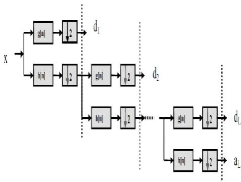
The signal is also decomposed simultaneously using a high-pass filter. The output gives the detail coefficients (from the high-pass filter) and approximation coefficients (from the low-pass filter). Applying this pair of filters to a time series leads to a first series which contains the trend (or slower dynamics) and a second one which contains the details (or fastest dynamics). This decomposition is repeated to further increase the frequency resolution and the approximation coefficients decomposition with low and high pass filters and then down sampled. This is represented as binary tree with nodes representing a sub space with different time frequency localization, the tree is known as bank. The filters h and g are low pass and high pass filters corresponding to the coefficients h(n) and g(n) respectively. Fig.1 illustrates L levels filter bank, which consists of a high-pass (details) filter (g) and a low-pass (approximation) filter (h). The original signal can be reconstructed from approximation and detail coefficients without losing information. The reconstruction process, also known as Inverse Discrete Wavelet Transform (IDWT) [13], is performed using undecimating and filtering. Undecimating consists of inserting zeros between values of carried out using synthesis filters based on decomposition filters.
The reconstructed signal is obtained by adding the outputs of synthesis filters. Fig (2) shows the reconstruction process.
Fig (1): L levels-Filter Bank
2.2 Multiwavelet Transform
As in the scalar wavelet case, the theory of multiwavelets is based on the idea of multiresolution analysis, analyzing the signal at different scales or resolutions. The difference is that multiwavelets have several scalling functions. The standard multiresolution has one scaling function
(
t
)
[14]. The multiwavelet two-scale equation resemble those for scalar wavelets:
k
k t k H
t) 2 (2 )
(
k
k t k G
t) 2 (2 )
(
Fig (2): Reconstruction process for DWT
(1)
(2)
(2)
(3)
[image:2.595.317.556.79.259.2] [image:2.595.311.547.423.679.2]One famous multiwavelet filter is the GHM filter proposed by [15]. Their system contains the two scaling functions
1(
t
)
and
2(
t
)
and the two wavelets
1(
t
)
and
2(
t
)
[16].According to Eqs.3 and 4, the GHM two scaling and wavelet functions satisfy the following two-scale dilation equations
) 2 ( 2 ) 2 ( 1 2 ) ( 2 ) ( 1 k t k t k k G t t
) 2 ( 2 ) 2 ( 1 2 ) ( 2 ) ( 1 k t k t k k H t t
For computing multiwavelet transform, a transform matrix can be written as follows [15]
Where Hi and Gi are the low- and high-pass filter impulse
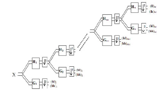
responses. The multiwavelet decomposition sub bands (after preprocessing and multiply the input signal by transform matrix) are shown in Fig (3). For multi-wavelet the
L
andH
have subscripts denoting the channel to which the data corresponds. For example, the sub band labeled LH corresponds to data from the second channel high pass filter and the first channel low-pass filter. This shows how a single level of decomposition is done. A single level of decomposition multiwavelet is roughly equivalent to two levels of scalar wavelet decomposition. Fig (4) show 1D MWT filter banks [16]Fig (3): Vector form of multiwavelet coefficients
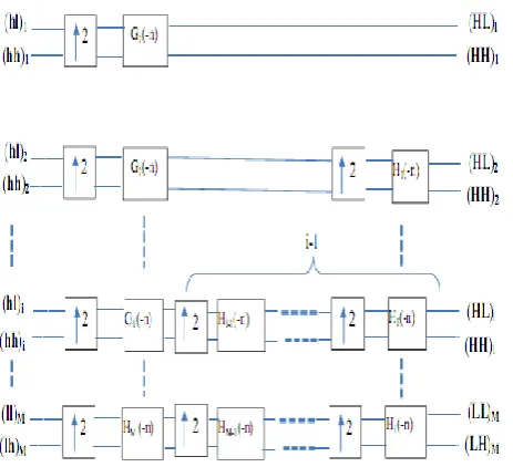
To reconstruct the time series signal, inverse multi wavelet must be taken for multiwavelet decomposition sub bands (LL,LH) and (HL,HH). By multiplying transposed transform matrix and multiwavelet subbands, the length of sub bands becomes equal to the original signal
length.
Fig (5) shows reconstruction Process for time series signal using 1D IMWT [16].Fig (4): M level 1D MWT filter banks
3. ECHO STATE NETWORK
Echo State Network was first field 0f reservoir technique proposed by Jaeger [17] to learn nonlinear systems and predict chaotic time series. Its basic idea is to use a large “reservoir” RNN as a supplier of interesting dynamics from which the desired output is combined [18]. Compared with traditional neural networks, ESN has the following advantages. First, the state of ESN contains information about the past input history in a way which reflects the recent history well and decays with the delay time. The feature of short-term memory solves the problem of adding memory and determining the range of time-delay values that many previous neural networks have and makes it suitable for stock prediction tasks. Second, the training of ESN is very simple and it can get the global optimal parameters. Therefore, ESN does not need to worry about local convergence that troubles conventional neural networks. Third, ESN performs much better than previous neural networks in stochastic time series prediction
.
The untrained part in ESN is called reservoir,and its weightsstay unchanged during training step.The trained part in ESN is called readout layer,the weights in this layer must be trained using one of training algorithms such as gradient descent algorithms or linear regression algorithms. Fig.6 show the basic network architecture considered here, the dotted lines represented the possible connections but not required .
.The real valued connection weights of ESN are collected in a N×M weight matrix Win = (
𝑤
𝑖𝑗𝑖𝑛) for the input weights, in an N×N matrix W = (wij) for the internal connections, in an L ×(M + N + L) matrix Wout = (
𝑤
𝑗𝑖𝑜𝑢𝑡) for the connections to theoutput units, and in a N×L matrix Wback = (
𝑤
𝑖𝑗𝑏𝑎𝑐𝑘) for the connectionsthat project back from the output to the internal units [7](5)
(6)
[image:3.595.296.548.86.232.2] [image:3.595.54.229.320.411.2]Fig (5):
Reconstruction Process for time series signal using 1D IMWTThe connections directly from the input to the output units and connection between output units are allowed.. No further conditions on the network topology induced by the internal weights W res are imposed (e.g., no layer
structure
). It will also not formally require, but generally intend that the internal connections Wres induce recurrent pathways between internal units .Wuthout further mention ,it will always assume real-valued inputs,weights,and activations.The activation of internal units is updated according to:And the output activation vector is updated according to:
4. PROPOSED FLOW DIAGRAM
In this work, the time series of the NNC 2010 is used as an illustration. The dataset of this signal can be found on the website http://www.neural-forecasting-competition.com. This time series data measured at different time frequencies. Therefore, it may contain a number of time series components including trend, seasonal and noise components. The general block diagram for proposed system of the prediction is shown in Fig.7. It is required to work in both the linear and nonlinear part of our recurrent neural network; the need is to normalize the time series to the interval [−1, 1]. Otherwise all neurons would be saturated and thus loosing information
Fig (6): The basic Echo State Network architecture
4.1 D
ecomposition
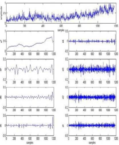
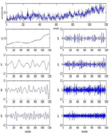
As shown in Fig. 7, the normalized time series is decomposed by means of wavelet and multiwavelet decomposition which results in a trend and a bunch of detail coefficients. The Daubechies (db4) and Meyer (dmey) wavelet filters were used to decompose time series signal up to the seventh level. Fig (8) and (9) show the time series of the NNC 2010 competition with its trend and detail coefficients using Db4 and Meyer filters in DWT respectively
. The functions of the Daubechies̕ system suffer from a major disadvantage for many applications they are discontinuous and cannot provide a good approximation for smooth functions. Meyer wavelet solves the problem of the discontinuity by means of interpolation [12]. GHM multiwavelet filter was used to decompose time series signal up t the seventh level. Fig (10) show the time series of the NNC 2010 competition with its components.
4.2 ESN predictor
The obtained components from decomposition step are predicted separately using Echo State Networks (ESN). Because of the nature of the task, generation of future time steps based on a learned history, the work will focus on the use of RC for recursive prediction [19]. This means that systems which have the delayed output feedback as an input to the reservoir will only be considered. Fig (11) shows reservoir computing for recursive prediction. In the present work, Training has been done in a supervised way by first driving the reservoir with teacher forced inputs
Secondly, the output layer trained by using linear regression methods. The neurons states of reservoir are updated by the following equations:
(8)
o(9)
[image:4.595.46.278.70.281.2] [image:4.595.319.537.86.278.2]Fig (7): Flow diagram for analysis and prediction of time series signals.
When testing the system, the teacher forced output feedback y (n) in equation (3.5) is replaced by the actual output
𝑦
(n) which is calculated by the following equation:Only the connections to the output, denoted by w
out
res
and wout
bias
, are changed during training in order to learn thedesired output function, the other matrixes are fixed and random. Because only the output weights are changed, training is extremely fast which can be an additional benefit in comparison with other methods. Additionally, the training of
the reservoir system does not suffer from local optima like other methods based on neural networks
Fig (8): Decomposition time series signal using DWT (Db4)
Finally, the predicted components are combined and rescaled in order to get a prediction of the given time series. The original signal can be obtained by summing up these predicted components [20].
where
aL: is the approximation component of L iterations.
dj: is the detail component of j iteration
The number of neurons in reservoir was set to 600 neurons and the connectivity of reservoir was set to 100% to make the network remember the input for very long time, To verify best stability for networks the spectral radius of reservoir varied from 0.1 to 0.9with a step of 0.1.
All the connections from the bias and output to the reservoir denoted by
𝑤
𝑏𝑖𝑎𝑠𝑟𝑒𝑠 and𝑤
𝑜𝑢𝑡𝑟𝑒𝑠 respectively, are drawn from a normal distribution [-1, 1]. The linear regression algorithm (LRA) was used to train the read out layer of ESN. The Tanh-Sigmoid function was used as the neural transfer function. The most important reason for choosing this activation function for the networks is that the Tanh-Sigmoid function f(x) is differentiable for all values of x, which allows the use of the powerful linear regression learning algorithm [7]
(11)
[image:5.595.319.527.75.330.2] [image:5.595.39.247.83.456.2]Fig (9): Decomposition time series signal using DWT (Meyer)
Fig (10) : Decompsition time series signal using MWT
(GHM)
5. RESULTS
For training and testing, the number of samples in each component signals has been divided into two parts: first part of these samples used for the training of the echo state network called training samples. The other part which has length equal to the desired prediction horizon used for the testing of the network called testing samples. Their resultant error is used to give the measure of generalization ability of the network.
The time series data contained 1181 samples. 50 and 100 samples are reserved from original data as the test for forecasting evaluation and comparison testing data.Table (1) shows the number of training and testing samples in each case.
Fig (11): Reservoir Computing for recursive prediction [16]
Table (1): Number of training and testing samples
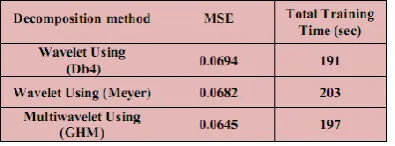
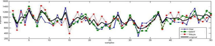
The spectral radius parameter was varied from 0.1 to 0.9 with a step of 0.1 to get better performance. The best results were in the spectral radius =0.9. Tables (2) and (3) show the results of prediction using LRA in read out layer of ESN with 50 and 100 samples as test respectively. Fig (12) and Fig (13) shows the original samples and predicted using Simple Echo State Network
[image:6.595.56.268.72.333.2] [image:6.595.318.548.253.441.2] [image:6.595.57.271.391.656.2] [image:6.595.335.531.514.587.2]Table (3): Results of prediction using 100 samples as test
6. CONCLUSION
The DWT-ESNs gave the worst results because the DWT gives approximate stationary details components, where the discontinuities appearance in these components increased the total training time and increased the mean square error. This can be attributed to the discrete jumps in the trend and many noisy detail coefficients that were derived from decomposition. As seen there was difference in the results of prediction using these two types of filters that returns to the difference in scaling functions used.
The main motivation of using the multiwavelet decomposition is the easy analysis of the obtained series. The GHM filter was used because this filter gives components which have few discontinuities, and more stationary in details components. Based on the results achieved, the combination of decomposition methods (DWT and MWT) with ESN had a great impact on the increasing accuracy of forcasting trend and seasonal time series.The comparison of the accuracy of the MWT system with the DWT system used in this paper gives a conclusion that the MWT system gives improved accuracy for time series prediction. Thus the MWT-ESNs gave the best results in our work.
8. REFERENCES
[1] Box, G.E.P. Jenkins, G.M. And Reinsel, G.C.1994. “Time Series Analysis. Forecasting and Control”, Prentice Hall.
[2] Winters, P.R.1960. “Forecasting Sales by Exponentially Weighted Moving Averages”, Journal Management Science, (6):pp. 324–342
[3] Bouqata, B., Bensaid, A., Palliam, R. and Gomez, A.F .2000.“Time Series Prediction Using Crisp and Fuzzy Neural Networks:A Comparative Study”, IEEE xplore, pp.170
[4] Suhartono, S.2006., “The Effect of Decomposition Method as Data Preprocessing on Neural Netorks Model for Forecasting Trend and Seasonal Time Series” , Institute of Research and Community Outreach - Petra Christian university, Vol. 8, No. 2, pp. 156-164.
[5] Turman, M. J. and Fine, T. L.1995. , “Sample Size Requirements for Feedforward Neural Networks”, Neural Information Processing System.Vol 7, pp. 327-334.
[6] Saad, E.W., Prokhorov, D. V. , and Wunsch, D.C II,1998. “Comparative Study of Stock Trend Prediction Using Time Delay Recurrent and Probabilistic Neural Networks”, IEEE Transactions on neural networks 9 (6): pp. 1456–1470
[7] Jaeger, H.2001., “The Echo State Approach to Analyzing and Training Recurrent Neural Networks”, Tech. Rep. GMD Report 148.
[8] Maass, W., Natschl¨ager, T. and H. Markram.2002. Real-time computing without stable states: A new framework for neural computation based on perturbations. Neural Computation, 14(11):2531–2560,.
[9] Verstraeten, D., Schrauwen, B., D’Haene, M. and Stroobandt, D.2007., “An experimental unification of reservoir computing methods”, Neural Networks, 20:391–403.
[10] Gao, X., Xiao, F., Zhang, J. and Cao, C.2004. , “Short-Term Prediction of Chaotic Time Series by Wavelet Networks”, 5th
World Congress on Intelligent Control and Automation, vol. 3, pp. 1931-1935.
[11] Lineesh, M. and Jessy, C.2010., “Analysis of Non-Stationary Time Series using Wavelet Decomposition”, Nature and Science, Vol. 8, pp. 53-59,
[12] Burrus, C. S., Gopinath , R. A. and Guo, H.1998., “ Introduction to Wavelets and Wavelet Transforms”, Prentice Hall.
[13] Garcia, A. and Gomez, P.2010 “Time Series Forecasting using Recurrent Neural Networks and Wavelet Reconstructed Signals”, 20th
International Conference on Electronics Communications and Computers, IEEE, pp.169-173.
[14] Ibraheem,A.K.2010. "Image Reconstruction Using Hybrid Transform", M.Sc. Thesis, Baghdad University, Eectrical Engineering Department.
[15] Geronimo, J., Hardian, D. & Massopust, P.1994."Fractal Function and Wavelet Expansion Based on Several Functions", J. Approx. Theory, Vol. 78, PP. 373-401.
[16] Strela, V. & Walden, A.T.1998. " Orthogonal and biorthogonal multiwavelets for signal denoising and image compression" Proc. SPIE, 3391: 96-107.
[17] Jaeger, H. and Haas, H.2004., “Harnessing Nolinearity: Predicting Chaotic Systems and Saving Energy in Wireless Communications”, Science, Vol.3.
[18] Jaeger, H.2002., “Short term memory in echo state networks”, Technical report, Report 152, GMD-German National Research Institute for Computer science.
[19] Wyffels, F., Schrauwen, B., and Stroobandt, D.2009., “Using Reservoir Computing in A Decomposition for Time Series Prediction, available at: http://reslab.elis.ugent.be/francis.
[image:7.595.60.258.97.170.2]Fig (12): The original & predicted samples (50 sample)
[image:8.595.70.511.74.168.2]