Power System Restoration Assessment Indices computation for a Restructured Power System with Bacterial Foraging Optimized Load Frequency Controller

Power System Restoration Assessment Indices

computation for a Restructured Power System with

Bacterial Foraging Optimized Load - Frequency

Controller

R.Thirunavukarasu

Assistant Professor Department of Electrical

Engineering Annamalai University,

Annamalainagar Tamilnadu, India.

B.Paramasivam

Assistant Professor Department of Electrical

Engineering Annamalai University,

Annamalainagar Tamilnadu, India,

I.A. Chidambaram

Professor Department of Electrical

Engineering Annamalai University,

Annamalainagar Tamilnadu, India,

ABSTRACT

This paper proposes, various design procedures for computing Power System Restoration Assessment Indices (PSRAI) for a Two-Area Hydro-Thermal Reheat Interconnected Power System (TAHTRIPS) in a restructured environment with a load-frequency controller optimized using Bacterial Foraging Optimization (BFO) algorithm. In the restructured scenario, as various types of apparatus with large capacity may enhance fast power consumption which causes serious problem in the frequency oscillations. The oscillation of system frequency may sustain and grow to cause stability problems in the system if no adequate damping is provided. The disturbances to the power system due to a small load change can even result in wide deviation in system frequency which is referred as load-frequency control problem. Quick system restoration is of prime importance not only based on the time of restoration and also stability limits also plays a very vital role in power system restoration problems due to unexpected load variations in power systems. The simple conventional Proportional plus Integral (P-I) controllers are still popular in power industry for frequency regulation as in case of any change in system operating conditions new gain values can be computed easily even for multi-area power systems. This paper focus on the computation of various PSRAI for TAH(with mechanical governor) -TRIPS and TAH (with Electric governor)- TRIPS unit based on the settling time concept, The design of the Proportional plus Integral (PI) controller gains are tuned using Bacterial Foraging Optimization (BFO) algorithm. These controllers are implemented to achieve a fast restoration time in the output responses of the system when the system experiences with various step load perturbations. In this paper the PRSAI are calculated for different types of possible transactions and the necessary remedial measures to be adopted are also suggested.

Keywords

Bacterial Foraging Optimization, Electric Governor, Frequency Control, Proportional plus Integral Controller, Restructured Power System, Power System Restoration Assessment Indices.

1.

INTRODUCTION

system. The importance of decentralized controllers for multi area load-frequency control in the restructured environment, where in, each area controller uses only the local states for feedback, is well known. The stabilization of frequency oscillations in an interconnected power system becomes challenging when implemented in the future competitive environment. So advanced economic, high efficiency and improved control schemes [8, 9] are required to ensure the power system reliability for which PSRAI can be used as a tool. In this paper various methodologies were adopted in computing Power System Restoration Assessment Indices (PSRAI) for Two-Area Hydro (with Mechanical/Electrical governor) Thermal Reheat Interconnected Power System (TAHTRIPS) in a restructured environment. With the various Power System Restoration Assessment Indices (Feasible Restoration Indices, Comprehensive Restoration Indices) the remedial measures to be taken can be adjudged like integration of additional spinning reserve, incorporation of effective intelligent controllers, load shedding etc.

In the early stages of power system restoration, the black start units are of the greatest interest because they will produce power for the auxiliaries of the thermal units without black start capabilities [9]. Under this situation a conventional frequency control i.e., a governor may no longer be able to compensate for sudden load changes due to its slow response. Therefore, in an inter area mode, damping out the critical electromechanical oscillations is to be carried out effectively in the restructured power system. Moreover, system frequency deviations should be monitored and remedial actions to overcome the frequency excursions are more likely to protect the system before it enters an emergency mode of operation. The restoration process of the bulk-power transmission system following a partial or a total blackout has two main issues during a restoration; these are voltage control and frequency control [10]. Special attention is therefore given to the behavior of network parameters, control equipments as they affect the voltage and frequency regulation during the restoration process which in turn reflects in PSRAI. During restoration due to wide fluctuations in the frequency and voltage it becomes very difficult to maintain the integrity in the system. Inability to control the frequency may lead to unsuccessful restoration. The repeated collapse of the system Islands due to tripping of generators due to either over frequency or under frequency condition causes delay in getting normalcy [10]

Now-a-days the complexities in the power system are being solved with the use of Evolutionary Computation (EC) such as Differential Evolution (DE) [11], Genetic Algorithms (GA), Practical Swarm Optimizations (PSO) [12] and Ant Colony Optimization (ACO) [13], which are some of the heuristic techniques having immense capability of determining global optimum. Classical approach based optimization for controller gains is a trial and error method and extremely time consuming when several parameters have to be optimized simultaneously and provides suboptimal result. Some authors have applied GA to optimize the controller gains more efficiently, but the premature convergence of GA degrades its search capability [14]. Recent research has brought out some deficiencies in using GA, PSO based techniques [14, 15]. The Bacterial Foraging Optimization [BFO] mimics how bacteria forage over a landscape of nutrients to perform parallel non gradient optimization [16]. The BFO algorithm is a computational intelligence based technique that is not affected

larger by the size and nonlinearity of the problem and can be convergence to the optimal solution in many problems where most analytical methods fail to converge. This more recent and powerful evolutionary computational technique BFO [16] is found to be user friendly and is adopted for simultaneous optimization of several parameters for both primary and secondary control loops of the governor.

To obtain the best convergence performance, an effective cost function is derived using the tie-line power and frequency deviations of the control areas and their rates of changes according to time integral. The main function of LFC is to regulate a signal called Area Control Error (ACE), which accounts for error in the frequency as well as the errors in the interchange power with neighboring areas. Conventional Load-Frequency Control uses a feedback signal that is either based on the Integral of ACE or is based on ACE and it’s Integral. These feedback signals are used to maneuver the turbine governor set points of the generators so that the generated power follows the load fluctuations, however continuously tracking load fluctuations definitely causes wear and tear on governor’s equipment, shortens their lifetime, and thus requires replacing them, which can be very costly. In this study, BFO algorithm is used to optimizing the Proportional plus Integral (PI) controller gains for the load frequency control of a Two-Area Hydro-Thermal Reheat Interconnected Power System (TAHTRIPS) in a restructured environment. Various case studies are analyzed to develop Power System Restoration Assessment Indices (PSRAI) namely, Feasible Restoration Index (FRI) and Complete Restoration Index (CRI) which are able to predict the normal operating mode, emergency mode and restorative modes of the power system.

2.

MODELING OF A TWO-AREA

HYDRO-THERMAL

REHEAT

INTERCONNECTED

POWER

SYSTEM

(TAHTRIPS)

IN

RESTRUCTURED

Load-Frequency Control (LFC) plays a very important role in power system and its main role is to maintain load-generation balance. Many investigations in the field of LFC for an interconnected system have been reported in literature over past few decades, which emphasizes on LFC pertaining to a thermal system and relatively a lesser attention has been contributed towards the LFC of a Hydro-Thermal system of widely different characteristics [17-22]. In this paper, investigation has been carried out for a TAHTIPS in which small perturbations was made to occur in area-1 and in area-2 and their impact on optimum selection of controller gain settling has been assessed based on the various Restoration Indices.

reality there will exist companies with combined or partial responsibilities. With the emergence of the distinct identities of GENCOs, TRANSCOs, DISCOs and the ISO, many of the ancillary services of a VIU will have a different role to play and hence have to be modeled differently. Among these ancillary service controls one of the most important services to be enhanced is the Load-frequency control [23]. The LFC in a deregulated electricity market should be designed to consider different types of possible transactions, such as poolco-based transactions, bilateral transactions and a combination of these two [24]. In the new scenario, a DISCO can contract individually with a GENCO for acquiring the power and these transactions will be made under the supervision of ISO. To make the visualization of contracts easier, the concept of “DISCO Participation Matrix” (DPM) is used which essentially provides the information about the participation of a DISCO in contract with a GENCO. In DPM, the number of rows has to be equal to the number of GENCOs and the number of columns has to be equal to the number of DISCOs in the system. Any entry of this matrix is a fraction of total load power contracted by a DISCO toward a GENCO. As a results total of entries of column belong to DISCOi of DPM is

∑

=1

icpfij . In this study

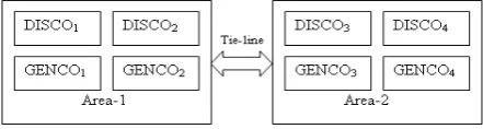
[image:3.595.60.281.399.458.2]

two-area interconnected power system in which each two-area has two GENCOs and two DISCOs. Let GENCO 1, GENCO 2, DISCO 1, DISCO 2 be in area 1 and GENCO 3, GENCO 4, DISCO 3, DISCO 4 be in area 2 as shown in Fig 1.The corresponding DPM is given as follows

Fig .1 Schematic diagram of two-area system in restructured environment

O C N E G cpf cpf cpf cpf cpf cpf cpf cpf cpf cpf cpf cpf cpf cpf cpf cpf O C S I D DPM                             = 44 43 42 41 34 33 32 31 24 23 22 21 14 13 12 11

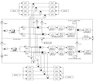
(1) Where cpf represents “Contract Participation Factor” and is like signals that carry information as to which the GENCO has to follow the load demanded by the DISCO. The linearized model of a two-area Hydro- Thermal reheat interconnected power system in deregulated environment is shown in Fig.2. The actual and scheduled steady state power flow through the tie-line is given as

j L i j ij j L i j ij scheduled

tie cpf P cpf P

P = ∆ − ∆

∆

∑∑

∑∑

= = = = − 4 3 2 1 2 1 4 3 , 2

1 (2)

∆Ptie₁−_2,actual =

(

2π T₁₂ /s

) (

∆F₁−∆F₂

)

(3)

And at any given time, the tie-line power error ∆P_{tie1−2,error} is defined as scheduled tie actual tie error

tie P P

P _1−2, =∆ _1−2, −∆ _1−2,

∆ (4)

The error signal is used to generate the respective ACE signals as in the traditional scenario [6]

ACE1=

β

1∆F1+∆Ptie1−2,error (5)

ACE₂ =

β

₂∆F₂ +∆P_{tie2−1,error} (6) For two area system as shown in Fig.1, the contracted power

supplied by ith _{GENCO is given as}

_j

DISCO j

j i i cpf PL

Pg = ∆

∆

∑

= = 4 1 (7)

Also note that ∆PL_1,LOC =∆PL₁+∆PL₂ and∆PL2,LOC =∆PL3 +∆PL4. In the proposed LFC implementation, contracted load is fed forward through the DPM matrix to GENCO set points. The actual loads affect system dynamics via the input ∆PL_,LOC to the power system blocks. Any mismatch between actual and contracted demands will result in frequency deviations that will drive LFC to re dispatch the GENCOs according to ACE participation factors, i.e., apf11, apf12, apf21 and apf22. The state space representation of

the minimum realization model of ‘

N

’ area interconnected power system may be expressed as [25].

x C y d u x x = Γ + Β + Α = • (8)

Where

x

=

[x

₁T

,

∆

p

_ei

...x

_(NT _-1)

,

∆

p

_e(N-1)

...x

T_N

]

T,

n

- state vector

∑

= − + = N i i N n n 1 ) 1 ( N P P u u

u=[ ₁,... _N]T =[∆ _C1... _CN]T, - Control input vector N

P P d

d

d D DN T

T

N] [ ... ] ,

,...

[ 1 = ∆ 1

= - Disturbance input

vectory=[y₁...y_N]T ,

2

N

- Measurable output vector where

A

is system matrix,

B

is the input distribution matrix,

Γ

is the disturbance distribution matrix,

C

is the control output distribution matrix,

x

is the state vector,

u

is the control vector and

d

is the disturbance vector consisting of load changes.

[image:4.595.148.449.112.371.2]

Fig. 2 Linerized model of a two-area hydro-Thermal reheat interconnected power system in restructured environment

3.

DESIGN OF DECENTRALIZED PI

CONTROLLERS

The proportional plus Integral controller gain values are tuned based on the cost function time of the output response of the system (especially the frequency deviation) and with these gain values the performance of the system is analyzed and the PSRAI are computed. In this case study the feedback controller adopted drives the plant to be controlled within a weighted sum of error and integral of that value i.e. it produces an output signal consisting of two terms one proportional to error signal and the other proportional to integral of error signal. The Integral Square Error (ISE) criterion [20] is used as the objective function and minimized using Bacterial Foraging Optimization Technique by effectively tunning the Proportional plus Integral gains (KPi, KIi) in the LFC loop.

Where,

_{U K ACE K ACE dt}

I

p −

∫

−

= 1 1

1

U2 =−Kp ACE2 −KI

∫

ACE2 dt (9)

Where, Kp - Proportional gain, KI- Integral gain, ACE - Area

Control Error, U1, U2 - Control input requirement of the

respective areas. The relative simplicity of this controller is a successful approach towards the zero steady state error in the frequency of the system.

4. BACTERIAL FORAGING

OPTIMIZATION (BFO) TECHNIQUE

4.1

.

Review of Bacterial Foraging Optimization

The BFO method was introduced by Possino [16]

motivated by the natural selection which tends to eliminate the animals with poor foraging strategies and favor those having successful foraging strategies. The foraging strategy is governed by four processes namely Chemotaxis, Swarming, Reproduction and Elimination and Dispersal. Chemotaxis process is the characteristics of movement of bacteria in search of food and consists of two processes namely swimming and tumbling. A bacterium is said to be swimming if it moves in a predefined direction, and tumbling if it starts moving in an altogether different direction. To represent a tumble, a unit length random direction

φ

(j)is generated. Let, “j” is the index of chemotactic step, “k” is reproduction step and “l” is the elimination dispersal event.

θ

_i

(

j

,

k

,

l

)

, is the position of ith bacteria at jth chemotactic step kth reproduction step and lth elimination dispersal event. The position of the bacteria in the next chemotatic step after a tumble is given by

(

j 1, k, l

)

i

(

j, k, l

)

C(i) (j)

i

_θ

_φ

θ

+ = + (10)

If the health of the bacteria improves after the tumble, the bacteria will continue to swim to the same direction for the specified steps or until the health degrades. Bacteria exhibits swarm behavior i.e. healthy bacteria try to attract other bacterium so that together they reach the desired location (solution point) more rapidly. The effect of swarming [19] is to make the bacteria congregate into groups and moves as

concentric patterns with high bacterial density. Mathematically swarming behavior can be modeled

(

)

(

)

(

(

)

)

(

)

(

)

(

)

(

)

∑

∑

∑

∑

∑

= =

= =

=

    

  

− −

− +

    

  

− −

− =

=

S i

p m

i m m repelent repelent

S i

p m

i m m attract attract

i S

i i cc

w h

d

l k j cc J l k j P J

1

2

1

1 1

2 1

exp exp

. . , ,

, ,

θ θ

θ θ ω

θ θ θ

(11) Where

CC

J

- Relative distance of each bacterium from the fittest bacterium

S

- Number of bacteria

p

- Number of parameters to be optimized

m

θ

- Position of the fittest bacteria

attract

d

,

ω

_attract,

h

_repelent,

ω

_repelent- different co-efficients representing the swarming behavior of the bacteria which are to be chosen properly In Reproduction step, population members who have sufficient nutrients will reproduce and the least healthy bacteria will die. The healthier population replaces unhealthy bacteria which get eliminated owing to their poorer foraging abilities. This makes the population of bacteria constant in the evolution process. In this process a sudden unforeseen event may drastically alter the evolution and may cause the elimination and / or dispersion to a new environment. Elimination and dispersal helps in reducing the behavior of stagnation i.e., being trapped in a premature solution point or local optima.

4.2.

Bacterial Foraging Algorithm

In case of BFO technique each bacterium is assigned with a set of variable to be optimized and are assigned with random values [

∆

] within the universe of discourse defined through upper and lower limits between which the optimum value is likely to fall. In the proposed method of proportional plus integral gain (KPi, KIi) (i=1, 2) scheduling, each bacterium

is allowed to take all possible values within the range and the cost objective function which is represented by Eq (9) is minimized. In this study, the BFO algorithm reported in [25] is found to have better convergence characteristics and is implemented as follows.

Step -1Initialization;

1. Number of parameter (p) to be optimized.

2. Number of bacterial (S) to be used for searching the total region.

3. Swimming length (Ns), after which tumbling of bacteria will be undertaken in a chemotactic loop 4. NC - the number of iteration to be undertaken in a chemotactic

5. Nre - the maximum number of reproduction to be undertaken.

6. Ned -the maximum number of elimination and dispersal events

to be imposed over bacteria

7. Ped - the probability with which the elimination and dispersal

events will continue.

8. The location of each bacterium P (1-p, 1-s, 1) which is specified by random numbers within

[-1, 1]

9. The value of C (i), which is assumed to be constant in this case for all bacteria to simplify the design strategy.

10. The value of d attract, W attract, h repelent and W repelent. It is to be

noted here that the value of dattract and h repelent must be same

so that the penalty imposed on the cost function through “JCC’’

of Eq (14) will be “0’’ when all the bacteria will have same value, i.e. they have converged. After initialization of all the above variables, keeping one variable changing and others fixed the value of “U’’ proposed in Eq (9) is obtained by running the simulation of system using the parameter contained in each bacterium. For the corresponding minimum cost, the magnitude of the changing variable is selected. Similar procedure is carried out for other variables keeping the already optimized one unchanged. In this way all the variables of step 1- initialization are obtain and are presented below

S = 6, Nc = 10, Ns = 3, Nre =15, Ned = 2, Ped =0.25, d attract

=0.01, w attract =0.04, h repelent =0.01, and w repelent =10, p = 2.

Step - 2Iterative algorithms for optimization:

This section models the bacterial population chemotaxis Swarming, reproduction, elimination, and dispersal (initially, j=k=l= 0) for the algorithm updating

θ

iautomatically results in updating of `P’.

1. Elimination –dispersal loop:

l

=

l

+

1

2. Reproduction loop:

k

=

k

+

1

3. Chemotaxis loop:

j

=

j

+

1

a) For i =1, 2…S, calculate cost for each bacterium i as follows.

• Compute value of cost

J

(

i

,

j

,

k

,

l

)

J (i,j,k,l) J(i,j,k,l) J ( i(j,k,l),P(j,k,l)) cc

sw = + θ

[i.e., add on the cell to cell attractant effect obtained through Eq (43) for swarming behavior to obtain the cost value obtained through Eq (9)].

Let

J

_last

=

J

_sw

(

i

,

j

,

k

,

l

)

to save this value since a better cost via a run be found.

End of for loop.

b) for i=1, 2….S take the tumbling / swimming decision.

Tumble: generate a random vector

∆

(

i

)

∈

ℜ

p with each element∆_m(i)m=1,2,...p, a random number ranges from [-1, 1].

Move the position the bacteria in the next chemotatic step after a tumble by Eq (10). Fixed step size in the direction of tumble for bacterium ‘i’ is considered

Compute

J

(

i

,

j

+

1

,

k

,

l

)

and then let Jsw(i,j+1,k,l)=J(i,j+1,k,l)+Jcc(θi(j+1,k,l),P(j+1,k,l)) (12)

Swim:

(i) Let m = 0 ; ( counter for swim length)

(ii) While m<Ns (have not climbed down too long)

Let m=m+1

If

J

_sw

(

i

,

j

+

1

,

k

,

l

)

<

J

_last (if doing better), let

)

,

,

1

,

(

J

_sw

i

j

k

l

J

_last

=

+

and let

(

)

(

)

( )

( )

( )

i

( )

i i i C l k j l k j

T i

i

∆ ∆

∆ +

=

+1, , θ , ,

θ (13) Where

( )

i

C

denotes step size;

∆

( )

i

Random vector;

∆

T

( )

i

Transpose of vector

∆

( )

i

.using Eq (13) the new

J

(

i

,

j

+

1

,

k

,

l

)

is computed. Else let m=Ns .This the end

of while statement

c). Go to next bacterium (i+1) is selected if i ≠S (i.e. go to step- b) to process the next bacterium

4. If j< Nc, go to step 3. In this case, chemotaxis is continued

since the life of the bacteria is not over. 5. Reproduction

a). For the given k and l for each i=1,2…S, let

)} , , , ( {

min _{{1... ]} J i j kl

Jihealth _{j N sw}

c

∈

= be the health of the

bacterium i (a measure of how many nutrients it got over its life time and how successful it was in avoiding noxious substance). Sort bacteria in the order of ascending cost Jhealth (higher cost

means lower health).

b). when Sr =S/2 bacteria with highest Jhealth values die

and other Sr bacteria with the best value split [and the copies

that are placed at the same location as their parent].

6. If k<Nre,go to 2; in this case, as the number of specified

reproduction steps have not been reached, so the next generation in the chemotactic loop is to be started.

7. Elimination –dispersal: for i = 1, 2… S with probability Ped,

eliminates and disperses each bacterium [this keeps the number of bacteria in the population constant] to a random location on the optimization domain.

5. SIMULATIONS RESULT AND

OBSERVATIONS

(Kp Ki) are tuned with BFO algorithm by optimizing the

solutions of control inputs for the various case studies as shown in Table 1. The results are obtained by MATLAB 7.01 software and 50 iterations are chosen for the convergence of the solution in the BFO algorithm. These PI controllers are implemented in a Two-Area Hydro-Thermal Interconnected restructured Power System for different type of transactions. The corresponding frequency deviations ∆f, tie- line power deviation ∆Ptie and

control input deviations ∆Pc are obtained with respect to time as

shown in figures 4-6. From the simulated results it is observed that the restoration process with the Hydro Turbines with Electric Governor ensures not only reliable operation but also provides a good margin of stability when compared with that of a Hydro plant with Mechanical Governor.

More over Power System Restoration Indices namely, Feasible Restoration Indices (FRI) when the system is operating in a normal condition with both units in operation and Comprehensive Restoration Indices (CRI) are one or more unit outage in any area are obtained as discussed. In this study GENCO-4 in area 2 is outage are considered. From these Restoration Indices the restorative measures like the magnitude of control input, rate of change of control input required can be adjudged.

5.1 Feasible Restoration Indices

5.1.1 Scenario 1: Poolco based transaction

The optimal Proportional plus Integral (PI) controller gains are obtained for TAHTIPS considering various case studies for framing the Feasible Restoration Indices (FRI) which were obtained based on Area Control Error (ACE) as follows:

Case 1: In the TAHTIPS considering Hydro (with

Mechanical/Electrical governor)-Thermal (HT) unit in area-1 and Thermal-Thermal (TT) units in area-2, for Poolco based transaction: in which the GENCOs in each area participate equally in LFC.If the load change occurs only in area 1. It denotes that the load is demanded only by DISCO 1 and DISCO 2. Let the value of this load demand be 0.1 p.u MW for each of them i.e. ∆PL1= 0.1 p.u MW, ∆PL 2= 0.1 p.u MW, ∆PL3 =

∆PL4= 0.0. DISCO Participation Matrix (DPM) referring to Eq

(14) is considered as [25]

     

 

     

 

=

0 0 0 0

0 0 0 0

0 0 5 . 0 5 . 0

0 0 5 . 0 5 . 0

DPM

(14)

Note that DISCO 3 and DISCO 4 do not demand power from any GENCOs and hence the corresponding contract participation factors (columns 3 and 4) are zero. DISCO 1 and DISCO 2 demand identically from their local GENCOs, viz., GENCO 1 and GENCO 2. Therefore, cpf11 = cpf12 = 0.5 and

cpf21 = cpf22 = 0.5. The frequency deviations (∆f )both area,

tie-line power deviation ∆Ptie and control input deviations ∆Pc as

shown the figure 4. The settling time (

ς

_s) and peak over /under shoot (Mp) of frequency deviations (∆f) in both the area and tie- line power deviation ∆Ptie were obtained from figures 4(a), 4(b)

and 4(c). From these values Feasible Restoration Indices are calculated as follows.

Step 5.1; The Feasible Restoration Index 1 (

ε

₁) is obtained from the ratio between the settling time of frequency deviation in area 1(

ς

_s1) and power system time constant (T_p1) of area 1

1 1 1

p s

T

FRI =

ς

(15)

Step 5.2; The Feasible Restoration Index 2 (

ε

₂) is obtained from the ratio between the settling time of frequency deviation in area 2 (

ς

_s2) and power system time constant(T_p2) of area 2

2 2 2

p s

T

FRI =

ς

(16)

Step 5.3; The Feasible Restoration Index 3 (

ε

₃) is obtained from the ratio between the settling time of tie –line power deviation (

ς

_s3) and synchronizing power coefficient T₁₂

12 3 3

T

FRI =

ς

s (17)

Step 5.4; The Feasible Restoration Index 4(

ε

₄) is obtained from the peak value of the frequency deviation ∆F₁(

ς

_p)response of area 1 with respect to the final value ∆F₁(

ς

_s)

FRI₄ =∆F₁(

ς

_p)−∆F₁(

ς

_s) (18)

Step 5.5; The Feasible Restoration Index 5(

ε

₅) is obtained from the peak value of the frequency deviation ∆F₂ (

ς

_p)response of area 2 with respect to the final value ∆F2 (

ς

s)

FRI₅=∆F₂(

ς

_p)−∆F₂(

ς

_s) (19) Step 5.6; The Feasible Restoration Index 6 (

ε

₆) is obtained from the peak value of the tie-line power deviation

)

( _p

tie

P

ς

∆ response with respect to the final value ∆P_tie (

ς

_s)

FRI6 =∆Ptie(

ς

p)−∆Ptie(

ς

s) (20)

Step 5.7; The Feasible Restoration Index 7 (

ε

7) is obtained from the rate of change of control input deviation requirement for area 1 using Lagrangian’s Interpolation method [27].

Time P FRI7 c1

∆

= (21)

Step 5.8; The Feasible Restoration Index 5 (

ε

₈) is obtained from the rate of change of control input deviation requirement for area 2 using Lagrangian’s Interpolation method.

Time P

FRI₈ =∆ c2 (22)

Case 2: This case is also a Poolco based transaction on

condition is indicated in the column entries of the DPM matrix and sum of the column entries is more than unity.

Case 3: It may happen that a DISCO violates a contract by

demanding more power than that specified in the contract and this excess power is not contracted to any of the GENCOs. This uncontracted power must be supplied by the GENCOs in the same area to the DISCO. It is represented as a local load of the area but not as the contract demand. Consider scenario-1 again with a modification that DISCO 1 demands 0.1 p.u MW of excess power i.e., ∆Puc, 1= 0.1 p.u MW and ∆Puc, 2 = 0.0 p.u

MW. The total load in area 1 = Load of DISCO 1+Load of DISCO 2 = ∆PL1 + ∆Puc1+∆PL2 =0.1+0.1+0.1 =0.3 p.u MW.

Case 4: This case is similar to Case 2 to with a modification that

DISCO 3 demands 0.1 p.u MW of excess power i.e., ∆Puc, 3= 0

p.u MW and., ∆Puc, 4 = 0 p.u MW. The total load in area 2

= Load of DISCO 3+Load of DISCO 4 = ∆PL1 +∆PL2 +∆Puc2

=0+0.1+0 =0.1 p.u MW.

Case 5: In this case which is similar to Case 3 with a

modification that DISCO 1 and DISCO 3 demands 0.1 p.u MW of excess power i.e., ∆Puc, 1= 0.1 p.u MW and ∆Puc, 3 = 0.1 p.u

MW. The total load in area 1 = Load of DISCO 1+Load of DISCO 2 = ∆PL1 + ∆Puc1 +∆PL2 =0.1+0.1+0.1 = 0.3 and total

demand in area 2 = Load of DISCO 3+Load of DISCO 4 = ∆PL3 + ∆Puc3 +∆PL4 =0+0.1+0 = 0.1 p.u MW

5.1.2 Scenario 2: Bilateral transaction

Case 6: Here all the DISCOs have contract with the GENCOs

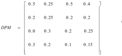
and the following DISCO Participation Matrix (DPM) be considered [25].

          

 

          

 

=

15 . 0 1 . 0 2 . 0 3 . 0

25 . 0 2 . 0 3 . 0 0 . 0

2 . 0 2 . 0 25 . 0 2 . 0

4 . 0 5 . 0 25 . 0 5 . 0

DPM

(23)

In this case, the DISCO 1, DISCO 2, DISCO 3 and DISCO 4, demands 0.15 p.u MW, 0.05 p.u MW, 0.15 p.u MW and 0.05 p.u MW from GENCOs as defined by cpf in the DPM

matrix and each GENCO participates in LFC as defined by the following ACE participation factor apf11 = apf12 = 0.5 and apf21

= apf22 = 0.5. The dynamic responses are shown in Fig. 5.

From this figure 5 the corresponding 5

4 3 2

1, FRI, FRI,FRI and FRI

FRI are calculated.

Case 7: For this case also bilateral transaction on TAHTIPS is

considered with a modification that the GENCOs in each area participate not equally in LFC and load demand is more than the GENCO in both the areas. But it is assumed that the load demand change occurs in both areas and the sum of the column entries of the DPM matrix is more than unity.

Case 8: Considering in the case 7 again with a modification that

DISCO 1 demands 0.1 p.u MW of excess power i.e., ∆Puc 1=

0.1 p.u.MW and ∆Puc 2 = 0.0 p.u MW. The total load in area 1

= Load of DISCO 1+Load of DISCO 2 = ∆PL1 + ∆Puc1+∆PL2

=0.15+0.1+0.05 =0.3 p.u MW and total load in area 2 = Load of DISCO 3+Load of DISCO 4 = ∆PL3 +∆PL4 =0.15+0.05 =0.2 p.u

MW.

Case 9 In the case which similar to case 8 with a modification

that DISCO 3 demands 0.1 p.u.MW of excess power i.e., ∆Puc, 3

= 0.1 p.u MW. The total load in area 1 = Load of DISCO 1+Load of DISCO 2 = ∆PL3 +∆PL4 =0.15+0.05 =0.2 p.u.MW

and total demand in area 2 = Load of DISCO 3+Load of DISCO 4 = ∆PL3 +∆PL4 +∆Puc3 =0.15+0.05+0.1 =0.3 p.u MW

Case 10: In the case which similar to case 9 with a modification

that DISCO 1 and DISCO 3 demands 0.1 p.u MW of excess power i.e., ∆Puc, 1= 0.1 p.u MW and ∆Puc, 3 = 0.1 p.u MW. The

total load in area 1 = Load of DISCO 1 + Load of DISCO 2 = ∆PL1 + ∆Puc1 +∆PL2 = 0.15+0.1+0.05 = 0.3 p.u MW and total

load in area 2 = Load of DISCO 3 + Load of DISCO 4 = ∆PL3 +

∆Puc3 +∆PL4 =0.15+0.1+0.05 = 0.3 p.u MW. For the Cases

1-10, the Feasible Restoration Indices are FRI1, FRI2, FRI3, FRI4,

FRI5, FRI6, FRI7 and FRI8 or ε1, ε2, ε3, ε4, ε5, ε6, ε7, and ε8 are

calculated are tabulated in Table 3 and Table 5. 5.2 Comprehensive Restoration Indices

Apart from the normal operating condition of the TAHTRIPS (with Mechanical/Electrical governor) few other case studies like one unit outage in an area, outage of one distributed generation in an area are considered individually. With the various case studies and based on their optimal gains the corresponding CRI is obtained as follows.

Case 11: In the TAHTIPS considering all the DISCOs have

contract with the GENCOs but GENCO4 is outage in area-2. In this case, the DISCO 1, DISCO 2, DISCO 3 and DISCO 4, demands 0.15 p.u MW, 0.05 p.u MW, 0.15 pu.MW and 0.05 pu.MW from GENCOs as defined by cpf in the DPM matrix

(23). The output GENCO4 = 0.0 p.u MW. The Comprehensive Restoration Indices

8 7

6 5 4 3 2

1, CRI, CRI,CRI,CRI,CRI,CRI andCRI

CRI ) are

obtained as

ε

₉,

ε

₁₀,

ε

₁₁,

ε

₁₂,

ε

₁₃,

ε

₁₄,

ε

₁₅,

ε

₁₆ and are tabulated in Table 6.

Case 12: Consider in this case which is same as Case 11 but

DISCO 1 demands 0.1 p.u MW of excess power i.e., ∆Puc 1= 0.1

p.u.MW and ∆Puc 2 = 0.0 p.u MW. The total load in

area 1 = Load of DISCO 1+Load of DISCO 2 = ∆PL1 +

∆Puc1+∆PL2 =0.15+0.1+0.05 =0.3 p.u MW and total load in

area 2 = Load of DISCO 3+Load of DISCO 4 = ∆PL3 +∆PL4

=0.15+0.05 =0.2 p.u MW

Case 13: This case is same as Case 11 with a modification that

DISCO 3 demands 0.1 p.u MW of excess power i.e., ∆Puc 3 =

0.1 p.u MW. The total load in area 1 = Load of DISCO 1+Load of DISCO 2 = ∆PL3 +∆PL4 =0.15+0.05 =0.2 p.u MW and total

demand in area 2 = Load of DISCO 3+Load of DISCO 4 = ∆PL3

[image:8.595.53.266.447.545.2]

Case 14: In this case which is similar to Case 11 with a modification that DISCO 1 and DISCO 3 demands 0.1 p.u MW of excess power i.e., ∆Puc 1= 0.1 p.u.MW and ∆Puc 3 = 0.1 p.u

MW. The total load in area 1 = Load of DISCO 1+Load of DISCO 2 = ∆PL1 + ∆Puc1 +∆PL2 = 0.15+0.1+0.05 = 0.3 p.u

MW and total load in area 2 = Load of DISCO 3+Load of DISCO 4 = ∆PL3 + ∆Puc3 +∆PL4 =0.15+0.1+0.05 = 0.3 p.u

MW. For the Case 11-14, the corresponding Comprehensive Restoration Indices

8 7

6 5 4 3 2

1, CRI , CRI ,CRI ,CRI ,CRI ,CRI andCRI

CRI are

calculated and tabulated in Table 6 5.3 Power System Restoration Assessment a) Based on Settling Time

(i) If

ε

₁,

ε

₂,

ε

₉,

ε

₁₀ ≥ 1 and

ε

₃,

ε

₁₁ ≥50 then more amount of distributed generation requirement is needed

b) Based on peak undershoot

(i)

If

ε

₄,

ε

₅,

ε

₁₂,

ε

₁₃ ≥1 and

ε

₆,

ε

₁₄ ≥0.15then the system is vulnerable and the system becomes unstable and may result to blackout.

(ii)

If 0.5≤

ε

4,

ε

5,

ε

12,

ε

13 ≤1then more amount of

distribution generation requirement is required but load shedding is also preferable.

(iii)

If 0.05≤

ε

6,

ε

14 ≤0.15then the FACTS devices

are required for the improvement of the tie-line power oscillations.

c) Based on control input deviation

(i) If 0.065≤

ε

₇,

ε

₈,

ε

₁₅,

ε

₁₆ ≤0.07 then more amount of distributed generation is needed.

[image:9.595.308.550.140.356.2]

(ii) If

ε

₇,

ε

₈,

ε

₁₅,

ε

₁₆ ≥0.07 then more amount of distributed generation as well as load shedding is preferable.

Table 1 Optimized Controller parameters of the TAHTRIPS (with Mechanical Hydro governor)

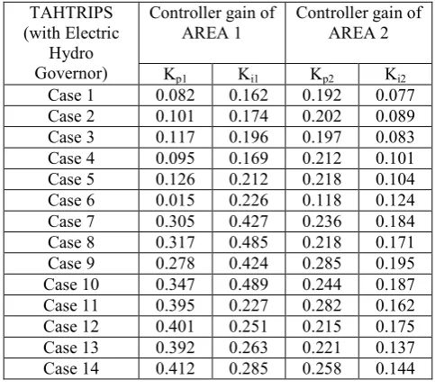
Table 2 Optimized Controller parameters of the TAHTRIPS (with Electric Hydro governor)

0 5 10 15 20 25 30 35

-0.7 -0.6 -0.5 -0.4 -0.3 -0.2 -0.1 0 0.1 0.2

Electric governor Mechanical governor

Fig.4 (a)∆F1 (Hz) Vs Time (s)

0 5 10 15 20 25 30 35

-0.4 -0.35 -0.3 -0.25 -0.2 -0.15 -0.1 -0.05 0 0.05

Electric governor Mechanical governor

Fig.4 (b)∆F2 (Hz) Vs Time (s)

TAHTRIPS (with Mechanical Hydro Governor)

Controller gain of AREA 1

Controller gain of AREA 2

Kp1 Ki1 Kp2 Ki2

Case 1 0.211 0.563 0.237 0.114

Case 2 0.234 0.312 0.245 0.169

Case 3 0.294 0.412 0.257 0.198

Case 4 0.256 0.456 0.312 0.201

Case 5 0.298 0.487 0.359 0.242

Case 6 0.264 0.412 0.215 0.169

Case 7 0.305 0.427 0.236 0.184

Case 8 0.317 0.485 0.218 0.171

Case 9 0.278 0.424 0.285 0.195

Case 10 0.347 0.489 0.244 0.187

Case 11 0.384 0.348 0.188 0.175

Case 12 0.401 0.351 0.215 0.205

Case 13 0.392 0.363 0.241 0.237

Case 14 0.412 0.385 0.278 0.244

TAHTRIPS (with Electric

Hydro Governor)

Controller gain of AREA 1

Controller gain of AREA 2

Kp1 Ki1 Kp2 Ki2

Case 1 0.082 0.162 0.192 0.077

Case 2 0.101 0.174 0.202 0.089

Case 3 0.117 0.196 0.197 0.083

Case 4 0.095 0.169 0.212 0.101

Case 5 0.126 0.212 0.218 0.104

Case 6 0.015 0.226 0.118 0.124

Case 7 0.305 0.427 0.236 0.184

Case 8 0.317 0.485 0.218 0.171

Case 9 0.278 0.424 0.285 0.195

Case 10 0.347 0.489 0.244 0.187

Case 11 0.395 0.227 0.282 0.162

Case 12 0.401 0.251 0.215 0.175

Case 13 0.392 0.263 0.221 0.137

Case 14 0.412 0.285 0.258 0.144

∆

F1

(

H

z)

Time (s)

∆

F2

(H

z)

0 5 10 15 20 25 30 35 -0.16

-0.14 -0.12 -0.1 -0.08 -0.06 -0.04 -0.02 0 0.02 0.04

Electric governor Mechanical governor

Fig.4 (c) ∆Ptie12 (p.u.MW) Vs Time (s)

0 5 10 15 20 25 30 35 40

-0.02 0 0.02 0.04 0.06 0.08 0.1 0.12 0.14 0.16 0.18

Electric governor Mechanical governor

Fig.4 (d) ∆Pc1 (p.u.MW) Vs Time (s)

0 5 10 15 20 25 30 35 40

-0.01 -0.008 -0.006 -0.004 -0.002 0 0.002 0.004 0.006 0.008 0.01

Electric governor Mechanical governor

Fig.4 (e) ∆Pc2 (p.u.MW) Vs Time (s)

Fig.4 Dynamic responses of the frequency deviations, tie- line power deviations and Control input deviations for a two-area hydro-thermal LFC system in the restructured scenario-1 (poolco based transactions

0 5 10 15 20 25 30 35 40

-0.7 -0.6 -0.5 -0.4 -0.3 -0.2 -0.1 0 0.1 0.2

Electric governor Mechanical governor

Fig.5 (a) ∆F1 (Hz) Vs Time (s)

0 5 10 15 20 25 30 35 40

-0.6 -0.5 -0.4 -0.3 -0.2 -0.1 0 0.1

Electric governor Mechanical governor

Fig.5 (b) ∆F2 (Hz) Vs Time (s)

0 5 10 15 20 25 30 35 40

-0.06 -0.04 -0.02 0 0.02 0.04 0.06 0.08 0.1

Electric governor Mechanical governor

Fig.5 (c) ∆Ptie12, actual (p.u.MW) Vs Time (s)

0 5 10 15 20 25 30 35 40

-0.12 -0.1 -0.08 -0.06 -0.04 -0.02 0 0.02 0.04

Electric governor Mechanical governor

Fig.5 (d) ∆Ptie12, error (p.u.MW) Vs Time (s)

∆

P

ti

e12

(

p

.u

.M

W

)

Time (s) Time (s)

∆

P

c1

(p

.u

.M

W

)

∆

P

c2

(p

.u

.M

W

)

Time (s)

∆

F1

(

H

z

)

Time (s)

∆

F2

(H

z)

Time (s)

Time (s)

∆

P

ti

e12

(

p

.u

.M

W

)

∆

P

ti

e12

,

er

ro

r

(

p

.u

.M

W

)

0 5 10 15 20 25 30 35 40 -0.05

0 0.05 0.1 0.15 0.2

Electric governor Mechanical governor

Fig.5 (e) ∆Pc1 (p.u.MW) Vs Time (s)

0 5 10 15 20 25 30 35 40 45 50

-0.02 -0.01 0 0.01 0.02 0.03 0.04 0.05 0.06

Electric governor Mechanical governor

Fig.5 (f) ∆Pc2 (p.u.MW) Vs Time (s)

Fig.5 Dynamic responses of the frequency deviations, tie- line power deviations, and Control input deviations for a two area HT system in the restructured scenario-2 (bilateral based transactions)

0 5 10 15 20 25 30 35 40 45 50

-1 -0.8 -0.6 -0.4 -0.2 0 0.2 0.4

Electric governor Mechanical governor

Fig.6 (a) ∆F1 (Hz) Vs Time (s)

0 5 10 15 20 25 30 35 40 45 50

-0.8 -0.7 -0.6 -0.5 -0.4 -0.3 -0.2 -0.1 0 0.1

Electric governor Mechnical governor

Fig.6 (b) ∆F2 (Hz) Vs Time (s)

0 5 10 15 20 25 30 35 40 45 50

-0.15 -0.1 -0.05 0 0.05 0.1

Electric governor Mechanical governor

Fig.6 (c) ∆Ptie12, actual (p.u.MW) Vs Time (s)

0 5 10 15 20 25 30 35 40 45 50

-0.2 -0.15 -0.1 -0.05 0 0.05

Electric governor Mechanical governor

Fig.6 (d) ∆Ptie12, error (p.u.MW) Vs Time (s)

0 5 10 15 20 25 30 35 40 45 50

0 0.05 0.1 0.15 0.2 0.25 0.3 0.35

Electric governor Mechanical governor

Fig.6 (e) ∆Pc1 (p.u.MW) Vs Time (s)

0 5 10 15 20 25 30 35 40 45 50

-0.02 -0.01 0 0.01 0.02 0.03 0.04 0.05

Electric governor Mechanical governor

Fig.6 (f) ∆Pc2 (p.u.MW) Vs Time (s)

Fig.6 Dynamic responses of the frequency deviations, tie- line power deviations and the Control input deviations for a two area HT system in the restructured scenario-3 (Contract violation)

∆

P

c1

(p

.u

.M

W

)

Time (s)

∆

P

c2

(p

.u

.M

W

)

Time (s)

Time (s)

∆

F1

(

H

z)

Time (s)

∆

F2

(H

z)

∆

P

ti

e12

(

p

.u

.M

W

)

Time (s)

∆

P

ti

e12

(

p

.u

.M

W

)

Time (s)

Time (s)

∆

P

c1

(p

.u

.M

W

)

Time (s)

∆

P

c2

(p

.u

.M

W

[image:12.595.107.490.135.319.2]

Table 3 Feasible Restoration Indices on TAHTRIPS (with Mechanical Hydro governor)

TAHTRIPS (with Mechanical

Hydro governor)

Feasible Restoration Indices (FRI) based on

Settling time(

ς

_s)

Feasible Restoration Indices (FRI) based on Peak over/ under shoot

(

M

_p

)

Feasible Restoration Indices (FRI) based

on control input deviation(∆P_c)

1

ε

ε

2

ε

3

ε

4

ε

5

ε

6

ε

7

ε

8

Case 1 0.975 0.945 45.96 0.431 0.351 0.125 0.051 --- Case 2 1.006 1.007 56.23 0.499 0.412 0.148 0.068 --- Case 3 1.425 1.234 55.51 0.952 0.583 0.141 0.071

[image:12.595.107.488.342.485.2]

Case 4 1.275 1.359 56.23 0.632 0.619 0.155 0.067 0.065 Case 5 1.512 1.475 59.63 0.985 0.712 0.159 0.069 0.066 Case 6 0.915 0.889 46.78 0.624 0.556 0.055 0.057 0.067 Case 7 1.624 1.322 48.69 0.883 0.654 0.069 0.064 0.062 Case 8 1.525 1.425 55.96 0.958 0.723 0.012 0.063 0.069 Case 9 1.278 1.534 55.51 0.952 0.883 0.021 0.071 0.074 Case 10 1.447 1.425 52.29 1.012 0.998 0.095 0.078 0.058 Table 4 Comprehensive Restoration Indices on TAHTRIPS (with Mechanical Hydro governor)

TAHTRIPS (with Mechanical

Hydro governor)

Comprehensive Restoration Indices (CRI) based on

Settling time(

ς

s)

Comprehensive Restoration Indices (CRI) based on Peak

over/ under shoot

(

M

_p

)

Comprehensive Restoration Indices

(CRI) based on control input

deviation(∆P_c)

9

ε

ε

10

ε

11

ε

12

ε

13

ε

14

ε

15

ε

16

Case 11 1.625 1.537 55.48 0.795 0.729 0.158 0.085 0.061

Case 12 1.724 1.637 56.39 0.895 0.621 0.162 0.091 0.041

Case 13 1.625 1.817 59.36 0.905 0.929 0.164 0.095 0.051

Case 14 1.947 1.825 59.29 1.012 1.128 0.169 0.111 0.058

Table 5 Feasible Restoration Indices on TAHTRIPS (with Electric Hydro governor)

TAHTRIPS (with Electric Hydro

governor)

Feasible Restoration Indices (FRI) based on

Settling time(

ς

_s)

Feasible Restoration Indices (FRI) based on Peak over/ under shoot

(

M

_p

)

Feasible Restoration Indices (FRI) based

on control input deviation(∆P_c)

1

ε

ε

₂

ε

₃

ε

₄

ε

₅

ε

₆

ε

₇

ε

₈

Case 1 0.906 0.942 42.96 0.418 0.317 0.091 0.051 --- Case 2 1.017 0.956 49.23 0.429 0.382 0.132 0.059 --- Case 3 1.315 1.142 53.12 0.852 0.483 0.135 0.068

[image:12.595.107.491.518.701.2]

[image:13.595.102.494.133.276.2]

Table 6 Comprehensive Restoration Indices on TAHTRIPS (with Electric Hydro governor)

TAHTRIPS (with Electric Hydro governor)

Comprehensive Restoration Indices (CRI) based on

Settling time(

ς

_s)

Comprehensive Restoration Indices (CRI) based on Peak

over/ under shoot

(

M

_p

)

Comprehensive Restoration Indices

(CRI) based on control input

deviation(∆P_c)

9

ε

ε

10

ε

11

ε

12

ε

13

ε

14

ε

15

ε

16

Case 11 1.525 1.417 54.36 0.665 0.719 0.148 0.075 0.055

Case 12 1.624 1.532 55.42 0.781 0.611 0.152 0.081 0.048

Case 13 1.525 1.711 58.16 0.813 0.939 0.154 0.089 0.048

Case 14 1.847 1.725 59.24 1.002 1.238 0.159 0.108 0.049

6. CONCLUSIONS

This paper proposes the design of various Restoration Assessment Indices which highlights the necessary requirements to be adopted in minimizing the frequency deviations, tie-line power deviation in a two-area interconnected Hydro-Thermal restructured power system to ensure the reliable operation of the power system. The PI controllers are designed using BFO algorithm and implemented in a Two-Area Two-Unit Hydro-Thermal Interconnected Restructured Power System without and with outraged conditions. The closed loop system was simulated and comparative studies of the output responses of the system for different type transactions conditions have been presented. From the simulated results it is observed that the restoration indices calculated for the Hydro Power Plants indicates that the Hydro plant with mechanical governor requires more sophisticated control for a better restoration of the power system output responses and to ensure improved Power System Restoration Assessment Indices (PSRAI) in order to provide good margin of stability than that of the Hydro plant with electric governor.

7. ACKNOWLEDGMENTS

The authors wish to thank the authorities of Annamalai University, Annamalainagar, Tamilnadu, India for the facilities provided to prepare this paper.

8. APPENDIX

A. Data for Thermal Reheat Power System [25]

Rating of each area = 2000 MW, Base power = 2000 MVA, fo = 60 Hz, R1 = R2 = R3 = R4 = 2.4 Hz / p.u.MW, Tg1 = Tg2 =

Tg3 = Tg4 = 0.08 sec, Tr1 = Tr2 = Tr1 = Tr2 = 10 sec, Tt1 = Tt2

= Tt3 = Tt4 = 0.3 sec, Kp1 = Kp2 = 120Hz/p.u.MW, Tp1 = Tp2 =

20 sec, β1 = β2 = 0.425 p.u.MW / Hz, Kr1 = Kr2 = Kr3 = Kr4 =

0.5, 2

π

T₁₂= 0.545 p.u.MW / Hz, a12 = -1, ∆PD1 = 0.01

p.u.MW

B. Data for Hydropower system with Mechanical governor [18] Tw = 1, a12 = -1; T1 = 48.7, T2 = 0.513,Tr = 5

C. Data for Hydro power system with Electric governor [19] Kd =4, Tw =1 s, Kp =1,, Ki =5

9. REFERENCES

[1] V.Donde, M.A.Pai, I.A.Hiskens, “Simulation and Optimization in an AGC System after Deregulation”, IEEE Transaction on Power System, 16(3), (2001), 481-489. [2] F.Liu, Y.H.Song, J.Ma, S.Mei, Q.Lu, “Optimal load-

Frequency control in restructured power systems”, IEE proceeding on Generation Transmission and Distribution, 150(1), (2003), 87-95.

[3] A.Demiroren, H.L.Zeynelgil, “GA application to optimization of AGC in three-area power system after deregulation”, Electrical Power and Energy System, 29(3), (2007), 230-240.

[4] H. Shayeghi, H.A. Shayanfar, O.P.Malik, Robust Decentralized Neural Networks Based LFC in a Deregulated Power System, Electric Power System Research, 77,(2007), 241-251.

[5] H. Shayeghi, H.A. Shayanfar, A. Jalili, “Load frequency Control Strategies: A state-of-the-art survey for the researcher”, Energy Conversion and Management, 50(2), (2009), 344-353.

[6] Ibraheem, P. Kumar, D.P.Kothari, “Recent philosophies of automatic generation control strategies in power systems”, IEEE Transactions on Power Systems, 20(1), (2005), 346-357.

[7] M.M.Adibi, J.N. Borkoski, R.J.Kafka and T.L. Volkmann,” Frequency Response of Prime Movers during Restoration”, IEEE Transactions on Power Systems 14(2), (1999), 751-756.

[8] M.M.Adibi and R.J.Kafka, “Power System Restoration Issues”, IEEE Computer Applications in Power, 4(2), (1991), 19-24.

[10] Jayesh J. Joglekar and Yogesh P. Nerkar, “A different approach in system restoration with special consideration of Islanding schemes”, Electrical Power and Energy Systems, 30, (2008), 519-524.

[11] CH. Liang, C.Y.Chung, K.P.Wong, X.Z.Duan, C.T.Tse, Study of Differential Evolution for Optimal Reactive Power Dispatch, IET Transactions on Generation Transmission and Distribution, 1(2007), 253-260.

[12] Y.Shi, R.C.Eberhart, Parameter Selection in PSO, “In Proceedings of 7th Annual Conference on Evolutionary Computation”, (1998), 591-601.

[13] M.Dorigo, M.Birattari, T.Stutzle, “Ant Colony optimization: artificial ants as a computational intelligence technique”, IEEE. Computational Intelligence Magazine, (2007), 28-39.

[14] Ghoshal, “Application of GA/GA-SA based fuzzy automatic control of multi-area thermal generating system”, Electric Power System Research, 70, (2004), 115-127. [15] M.A.Abido, “Optimal design of power system stabilizers

using particle swarm optimization”, IEEE Transaction. Energy Conversion, 17(3), (2002), 406-413.

[16] K.M.Passino, “Biomimicry of bacterial foraging for distributed optimization and control”, IEEE Control Syst Magazine, 22 (3), (2002), 52-67.

[17] M.L. Kothari, B.L.Kaul and J.Nanda, “Automatic generation control of hydro-thermal system”, Journal of Institution of Engineers (India), 61, (1980), 1-4

[18] Prabhat Kumar, K.E. Hole and R.P. Aggarwal, “Design of a decentralized AGC regulation for two-area hydro-thermal power system”, Journal of Institution of Engineers (India), Vol.63, pt EL., pp.304-309, 1983

[19] O.P.Malik, G.S. Hope, S.C. Tripathy and N.Mital, “Decentralized sub-optimal load-frequency control of a hydro-thermal power system using state variable model”, Electric power system research, Vol.8, pp.237-247, 1984/85.

[20] Nanda J, Mangala, A, Suri, S, “Some new findings on automatic generation control of an interconnected hydrothermal system with conventional controllers”, IEEE Transactions of Energy Conversion, Vol.21,pp.187-194, March 2006.

[21] Surya Prakash, S.K.Sinha, “Application of artificial intelligence in load frequency control of interconnected power system”, International Journal of Engineering, Science and Technology, Vol.3, No.4, pp.264-275, 2011 [22] Janardan Nanda, Mishra.S., Lalit Chandra Saikia, “Maiden

Application of Bacterial Foraging-Based optimization technique in multi-area Automatic Generation Control”, IEEE Transaction on Power System, 24(2), (2009), 602-609.

[23] S.Farook, P.Sangameswara Raju, “AGC controllers to optimize LFC regulation in deregulated powersystem”, International Journal of Advances in Engineering & Technology, IJAET ISSN:2231-1963, Nov 2011, Vol.1, Issue 5, pp. 278-289.

[24] C.Srinivasa Rao, “Implementation of Load Frequency Control of Hydrothermal System under Restructed Scenario Employing Fuzzy Controlled Genetic Algorithm”, International Journal of Advanced Research in Electrical Electronics and Instrumentation Engineering, ISSN: 2278-8875,July 2012, Vol.1, Issue 1, pp.1-6.

[25] B.Paramasivam and I.A.Chidambaram, “Bacterial Foraging Optimization Based Load-Frequency Control of Interconnected Power Systems with Static Synchronous Series Compensator”, International Journal of Latest Trend in Computing, Vol 1, Issue 2, pp.7-15, 2010.

[26] K.Ogatta, Modern Control System Engineering, 5th _Edition,

Pearson Education, New Jessey, 2010.

[27] M.Shanthakumar, Computer Based Numerical Analysis, Khanna Publishers, New Delhi, 1999.

10. AUTHORS’ PROFILE

R.Thirunavukarasu (1977) received Bachelor of Engineering

in Electrical and Electronics Engineering (2001),Madurai kamaraj university Madurai, Master of engineering in power system (2004) from Annamalai university, Annamalainagar, Chidambaram. currently working as an Assistant professor in the department of electrical engineering, Annamalai university since 2007. He is currently working towards the Ph.D degree. His research interest are power system operation and Control, Electrical Measurements.

B.Paramasivam (1976) received Bachelor of Engineering in

Electrical and Electronics Engineering (2002), Master of Engineering in Power System Engineering (2008) and he is working as Assistant Professor in the Department of Electrical Engineering, Annamalai University, Annamalainagar-608002, Tamilnadu, India. He is currently pursuing Ph.D degree in Electrical Engineering at Annamalai University, Annamalainagar. His research interests are in Power System, Control Systems, Electrical Measurements.

I.A.Chidambaram (1966) received Bachelor of Engineering in