Transmuted Generalized Linear Exponential Distribution

(1)

Transmuted Generalized Linear Exponential

Distribution

I. Elbatal

Institute of Statistical Studies and Research Department of Mathematical Statistics

Cairo University.

L.S. Diab

College of Science for (girls)

Dept. of Mathematics, Al-Azhar University, Egypt.

N. A. Abdul Alim

College of Science Dept. of Mathematics Al-Azhar University, Egypt.

ABSTRACT

The linear exponential distribution is a very well-known distribu-tion for modeling lifetime data in reliability and medical studies.We introduce in this paper a new four-parameter generalized version of the transmuted generalized linear exponential distribution.We pro-vide a comprehensive account of the mathematical properties of the new distributions. In particular, A closed-form expressions for the density, cumulative distribution ,quantile and median of the distri-bution is given. Also, therthorder moment and moment

generat-ing function are derived. The maximum likelihood estimation of the unknown parameters is discussed. Real data are used to determine whether the TGLED is better than other well-known distributions in modeling lifetime data or not.

Keywords:

Transmuted generalized linear exponential distribution, quantile and median, Maximum likelihood estimation, Moments.

1. INTRODUCTION AND MOTIVATION

The linear exponential distribution is also known as the Linear Fail-ure Rate distribution , having exponential and Rayleigh distribu-tions as special cases, is a very well-known distribution for model-ing lifetime data in reliability and medical studies. It is also models phenomena with increasing failure rate. However, theLE distribu-tion does not provide a reasonable parametric fit for modeling phe-nomenon with decreasing, non linear increasing, or non-monotone failure rates such as the bathtub shape, which are common in firm ware reliability modeling, biological studies, see Lai et al. (2001) and Zhang et al. (2005).

A new generalization of the linear exponential distribution is gen-eralized linear exponential(GLE)distribution. This distribution is important since it contains as special sub-models some widely well known distributions. It also provides more flexibility to ana-lyze complex real data sets. (see Mahmoud and Alam (2010)). A random variableX is said to have the generalized linear expo-nential distribution with three parametersα, βandθ, if it has the cumulative distribution function

G(x, α, β, θ) = 1−e−(αx+β₂x2₎θ

, x >0, α, β, θ >0, (1)

and the corresponding probability density function (pdf) is given by

g(x, α, β, θ) = θ(α+βx)(αx+β 2x

2₎θ−1_e−(αx+β₂x2₎θ

,

x >0, α, β, θ >0. (2) The quality of the procedures used in statistical analysis depends heavily on the assumed probability model or distributions. Because of this, considerable effort over the years has been expended in the development of large classes of standard probability distributions along with relevant statistical methodologies. In fact, the statistics literature is filled with hundreds of continuous univariate distribu-tions. However, in recent years, applications from the environmen-tal, financial, biomedical sciences, engineering among others, have further shown that data sets following the classical distributions are more often the exception rather than the reality. Since there is a clear need for extended forms of these distributions a significant progress has been made toward the generalization of some well-known distributions and their successful application to problems in areas such as engineering, finance, economics and biomedical sci-ences, among others.

In this article we use transmutation map approach suggested by Shaw and Buckley (2007) to define a new model which general-izes the generalized linear exponential Distribution . We will call the generalized distribution as the transmuted generalized linear exponential distribution(TGLED) distribution. According to the

Quadratic Rank Transmutation Map,(QRTM), approach the cumu-lative distribution function (cdf) satisfy the relationship

F2(x) = (1 +λ)F1(x)−λF1(x)2 (3) which on differentiation yields,

f2(x) =f1(x) [(1 +λ)−2λF1(x)] (4) wheref1(x)andf2(x)are the corresponding pdfs associated with cdfF1(x)andF2(x)respectively and−1≤λ≤1. An extensive information about the quadratic rank transmutation map is given in Shaw and Buckley (2007).

We will use the above formulation for a pair of distributionsF(x)

andG(x)whereG(x)is a sub-model ofF(x). Therefore, a random variableXis said to have a transmuted probability distribution with cdfF(x)if

F(x) = (1 +λ)G(x)−λG(x)2_,_{|λ| ≤}₁_,

(2)

whereG(x)is the cdf of the base distribution. Observe that atλ

= 0we have the distribution of the base random variable. Many authors dealing with the generalization of some well- known distributions . Aryal and Tsokos (2009) defined the transmuted generalized extreme value distribution and they studied some ba-sic mathematical characteristics of transmuted Gumbel probability distribution and it has been observed that the transmuted Gumbel can be used to model climate data. Also Aryal and Tsokos (2011) presented a new generalization of Weibull distribution called the transmuted Weibull distribution . Recently, Aryal (2013) proposed and studied the various structural properties of the transmuted Log-Logistic distribution. and Muhammad khan and King (2013) in-troduced the transmuted modified Weibull distribution which ex-tended recent development on transmuted Weibull distribution by Aryal et al. (2011). and they studied the mathematical properties and maximum likelihood estimation of the unknown parameters.In the present study we will provide mathematical formulation of the transmuted generalized linear exponential distribution (TGLED)

distribution and some of its properties.

Merovci and Elbatal (2013) introduce a new lifetime distribution by transmuted and compounding Lindley and geometric distribu-tions named transmuted Lindley geometric distribution.They de-rive expansions for moments and for the moment generating func-tion. The estimation of parameters is approached by the method of maximum likelihood, also the information matrix is derived. An application of the transmuted Lindley geometric distribution to real data. Elbatal (2013) proposed a functional composition of the cu-mulative distribution function of one probability distribution with the inverse cumulative distribution function of another is called the transmutation map.He used the quadratic rank transmutation map (QRTM) in order to generate a flexible family of probability dis-tributions taking modified inverse weibull distribution as the base value distribution by introducing a new parameter that would offer more distributional flexibility. It will be shown that the analytical results are applicable to model real world data. Elbatal and Aryal (2013) presented the transmuted additive Weibull distribution, that extends the additive Weibull distribution and some other distribu-tions they used the quadratic rank transmutation map (QRTM) pro-posed by Shaw & Buckley( 2007) in order to generate the trans-muted additive Weibull distribution. Various structural properties of the new distribution including the explicit expressions for the mo-ments,random number generation and order statistics are derived. Maximum likelihood estimation of the unknown parameters of the new model for complete sample is also discussed. It will be shown that the analytical results are applicable to model real world data. The rest of the paper is organized as follows. In Section 2 we demonstrate transmuted probability distribution, and we present the flexibility of the subject distribution and some special sub-models. The reliability functions of the subject model are given in Section 3. In Section 4 we studied the statistical properties include quantile functions, moments, moment generating function . The minimum , maximum and median order statistics models are discussed in Sec-tion 5. Finally, In SecSec-tion 6 we demonstrate the maximum likeli-hood estimates and the asymptotic confidence intervals of the un-known parameters. Finally, some lifetime data sets are used to illus-trate that the generalized linear exponential distribution (TGLED) can used for the data under analysis, comparing with some known distributions.

2. TRANSMUTED GENERALIZED LINEAR

EXPONENTIAL DISTRIBUTION

In this section we studied the transmuted generalized linear expo-nential distribution(TGLED)and the sub-models of this

distribu-tion. Now using??and??we have the cdf of transmuted general-ized linear exponential distribution

FT GLE = (1 +λ)

1−e−(αx+β₂x2₎θ

−λ1−e−(αx+β₂x2₎θ2

,

=

h

1−e−(αx+β2x2)θ i h

1 +λe−(αx+β2x2)θ i

(6) whereα,βare the scale parameters ,θis shape parameter repre-senting the different patterns of the transmuted generalized linear exponential distribution andλis the transmuted parameter. The re-strictions in equation (6) on the values ofα, β, θandλare always the same. The probability density function (pdf) of the transmuted generalized linear exponential distribution is given by

fT GIE(x) = θ(α+βx)((αx+

β

2x

2

)θ−1e−(αx+β2x2)θ× h

1−λ+ 2λe−(αx+β2x2)θ i

. (7)

The transmuted generalized linear exponential distribution is very flexible model that approaches to different distributions when its parameters are changed.

(i) Ifλ= 0we get the generalized linear exponential distribution GLED(α, β, θ).

(ii) Ifα= 1

σ, β = 0we get the transmuted Weibull distribution

TW D(λ, σ, θ).

(iii) Ifλ=β= 0, α=1

σwe get theWeibull distributionW(σ, θ).

(iv) Ifθ= 1we get the transmuted linear exponential distribution TLED(λ, α, β)

(v) If θ = 1, α = 0 we get the transmuted Rayleigh distributionTRD(λ, β)

(vi) Ifθ = 1, α =λ = 0we get the Rayleigh distributionRD

[image:2.595.335.536.493.692.2]

(β).

(3)

[image:3.595.86.270.66.267.2]

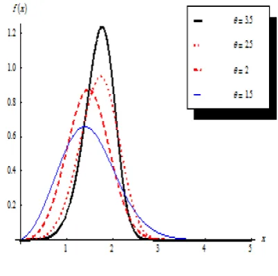
Fig. 1. Effect of shape parameterθon the TGLED PDF

3. RELIABILITY ANALYSIS

The transmuted generalized linear exponential distribution can be a useful characterization of life time data analysis. The reliabil-ity function(RF)of the transmuted generalized linear exponential distribution is denoted byRTGLED(x)also known as the survivor

function and is defined as RTGLED(x)

= 1−FTGLED(x)

= 1−h1−e−(αx+β2x2)θ i h

1 +λe−(αx+β2x2)θ i

. (8) Figure 2 (a) and (b) represent the CDF and RF respectively for different values of shape parameterθ.

Fig. 2(a) CDF Fig. 2(b) RF

It is important to note thatRTGLED(x) +FTGLED(x) = 1. One

of the characteristic in reliability analysis is the hazard rate function (HRF) defined by

hT GIE(x)

= fTGLED(x)

1−FTGLED(x)

= θ(α+βx)((αx+ β

2x

2₎θ−1_e−(αx+β₂x2₎θ

)

1−h1−e−(αx+β₂x2₎θi h

1 +λe−(αx+β₂x2₎θi

.

×

h

1−λ+ 2λe−(αx+β₂x2)θi

1−h1−e−(αx+β₂x2₎θi h

. (9)

It is important to note that the units forhT GIE(x)is the probability

of failure per unit of time, distance or cycles. These failure rates are defined with different choices of parameters.The cumulative hazard function of the transmuted generalized inverted exponential distri-bution is denoted byHT GIE(x)and is defined as

HT GIE(x) =−ln

h

1−e−(αx+β₂x2₎θi h

(10) It is important to note that the units forHT GIE(x)is the cumulative

[image:3.595.340.557.72.346.2] [image:3.595.73.272.471.632.2]

(4)

Fig. 3(a)

Fig. 3(b)

Fig. 3(c)

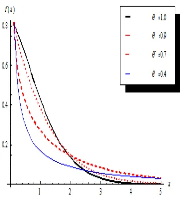
Fig. (3) Effect of shape parameterθ on the hazard rate function (HRF) of the TGLED.

THEOREM 1. The hazard rate function of the transmuted gen-eralized linear exponential distribution has the following proper-ties

(i) Ifλ= 0we get the failure rate is same as theGLED(α, β, θ). (ii) Ifα = 1

σ, β = 0we get the the failure rate is same as the

TW D(λ, σ, θ).

(iii) Ifλ=β= 0, α= 1

σ we get the the failure rate is same as the

W(σ, θ).

(iv) If θ = 1 we get the the failure rate is same as the TLED(λ, α, β).

PROOF. The hazard function (HF) of the transmuted general-ized linear exponential distribution is given in equation (9) has the special cases with different choice of parameters:

(i) Ifλ= 0we get the failure rate is same as theGLED(α, β, θ)

hGLED=θ(α+βx)((αx+

β

2x

2₎θ−1

(ii) Ifα = 1

σ, β = 0we get the the failure rate is same as the

TW D(λ, σ, θ).

hTW D(x) =

θx σ (

x σ)

θ−1_e−(x_σ)θh₁₋_λ_{+ 2}_λe−(x_σ)θi

1−

1−e−(x_σ)θ

1 +λe−(_σx)θ

. .

(iii) Ifλ=β= 0, α= 1

σ we get the the failure rate is same as the

W(σ, θ)

h_{W D}(x) = θx

σ( x σ)

θ−1_e−(x σ)θ

1−

1−e−(_σx)θ

(iv) If θ = 1 we get the the failure rate is same as the TLED(λ, α, β)

h_{T LED}(x) =

(α+βx)e−(αx+β₂x2₎h

1−λ+ 2λe−(αx+β₂x2₎i

1−h1−e−(αx+β₂x2₎i h

1 +λe−(αx+β₂x2₎i

.

4. STATISTICAL PROPERTIES

This section is devoted to study statistical properties for the trans-muted generalized linear exponential, specifically Quantile func-tion ,median, moments, moment generating funcfunc-tion.

4.1 Quantile and Median

The quantilexqof theTGLED(α, β, θ,λ, x)is real solution of the

following equation

xq=

−α+

r

α2_{+ 2}_βh₋_ln(λ−1)+ √

(λ+1)2−4λq

2λ

i1θ

β (11)

The above equation has no closed form solution inxq, so we have

[image:4.595.107.567.37.734.2] [image:4.595.312.553.242.518.2]

(5)

4.2 Random Number Generation

The random number generation asxof theTGLED(α, β, θ,λ, x)

is defined by the following relation h

1−e−(αx+β2x2) i h

1 +λe−(αx+β2x2) i

=ϕwhereϕ∼U(0,1)

thus

x=

−α+

r

α2_{+ 2}_βh₋_ln(λ−1)+ √

(λ+1)2−4λϕ

2λ

i1θ

β . (12)

4.3 Moments

In this subsection, we derive therthmoments and moment

gener-ating functionMX(t)of theT GLE. The following theorem gives

therthmoment(µr)of theTGLED(α, β, θ,λ, x.)

THEOREM 2. IfXhasT GLE, then therthmoment ofX, r= 1,2, ....has the following form:

µ0_r = r X i=0 ∞ X j=0

(−1)i+j

r i

r−i

2 j

2

r−i

2 −j_×

αi+2j 1 βr+2i+j

n

(1−λ)Γ(r−i 2θ −

j θ + 1)

+λ2−(r+22θθ−i)+ j θ_Γ(r−i

2θ − j θ + 1)

o

.

PROOF. We start with the well known definition of therth

mo-ment of the random variableXwith pdf of transmuted generalized linear exponential given by

µ0r = E(X r

)

=

Z ∞

0

xrfT GLE(x)dx

=

(1−λ)

Z ∞

0

xr_θ₍_α₊_βx₎₍_αx₊β 2x

2₎θ−1_e−(αx+β₂x2₎θ

+ 2λ

Z ∞

0

θxr₍_α₊_βx₎₍_αx₊β 2x

2₎θ−1_e−2(αx+β₂x2)θ

×dx (13)

Now we define the following substitutiony = (αx+β₂x2₎θ _this

implies thatdy=θ(αx+β₂x2₎θ−1₍_α₊_βx₎_dx._Clearly,

x=−α+

p

α2_{+ 2}_βy1_θ β

Thus

µ0_r = (1−λ)

( Z ∞

0 "

−α+pα2_{+ 2}_βy1_θ β

#r

e−y

+ 2λ

"

−α+pα2_{+ 2}_βy1θ

β

#r

e−2y

)

dy, (14)

by using the binomial series expansion ofh−α+pα2_{+ 2}_βy1_θi

r

we get

−α+

q

α2_{+ 2}_βy1θ

r

= r

X

i=0

(−1)i

r i αi

α2+ 2βy1θ

r−2i

,

(15) and

α2+ 2βy1θ

r−2i

= (2β)r−2i_yr2−θi

∞

X

j=0

(−1)j

_r−i

2 j

α2

2βy1θ

j

,

(16) substituting from (15) and (16) into (14), we have the following

µ0_r = r X i=0 ∞ X j=0

(−1)i+j

r i

r−i

2 j

2

r−i

2 −j

αi+2j 1

βr+2i+j

×

Z ∞

0 yr2−θi−

j θe−y2λ

βr

Z ∞

0 yr2−θi−

j θe−2y

dy = r X i=0 ∞ X j=0

(−1)i+j

r i

r−i

2 j

2

r−i

2 −j

αi+2j 1

βr+2i+j

×

n

(1−λ)Γ(r−i 2θ −

j θ + 1)

+λ2−(r+22θθ−i)+ j θ_Γ(r−i

2θ − j θ+ 1)

o

(17) therefore

µ0r=Ci,jΓ(

r−i

2θ − j θ + 1)

"

1−λ+λ

₁

2

r2−θi− j θ+1

#

(18) where

Ci,j= r X i=0 ∞ X j=0

(−1)i+j

r i

r−i

2 j

2

r−i

2 −j

αi+2j 1 β3r2+i+j which completes the proof .

THEOREM 3. IfX hasT GLE, then the moment generating functionMX(t)has the following form

MX(t) = Ci,j ∞

X

r=0 tr

r!Γ(

r−i

2θ − j θ+ 1)×

"

1−λ+λ1

2

r2−θi− j θ+1

#

PROOF. We start with the well known definition of the moment generating function given by

MX(t) = E(etx)

=

Z ∞

0

etxfT GLE(x)dx

= Z ∞ 0 ∞ X r=0 tr_xr

r! fT GLE(x)dx

= ∞

X

r=0 tr

r!µ

0

(6)

= Ci,j ∞

X

r=0 tr

r!Γ(

r−i

2θ − j θ + 1)×

"

1−λ+λ

₁

2

r2−θi− j θ+1

#

(19)

which completes the proof.

5. ORDER STATISTICS

The order statistics have many applications in reliability and life testing. The order statistics arise in the study of reliability of a sys-tem. LetX1, X2, ..., Xnbe a simple random sample fromTGLED (α, β, θ, λ, x) with cumulative distribution function and proba-bility density function as in (6) and (7), respectively. LetX(1:n) ≤X(2:n)≤...≤X(n:n)denote the order statistics obtained from this sample. In reliability literature,X(i:n)denote the lifetime of an

(n−i+ 1)−out−of−nsystem which consists ofnindependent and identically components. Then the pdf ofX(i:n),1≤i≤nis given by

fi::n(x) =

1

β(i, n−i+ 1)[F(x,Φ)] i−1

[1−F(x,Φ)]n−if(x,Φ)

(20) whereΦ = (α, β, θ,λ,)also, the joint pdf ofX(i:n), X(j:n)and

1≤i≤j≤nis

fi:j:n(xi, xj) = C[F(xi)]i −1

[F(xj)−F(xi)]j −i−1_×

[1−F(xj)]n −j

f(xi)f(xj) (21)

where C

C= n!

(i−1)!(j−i−1)!(n−j)!

We defined the first order statisticsX(1)=M in(X1, X2, ..., Xn),

the the last order statistics asX(n) =M ax(X1, X2, ..., Xn)and

median orderXm+1.

5.1 Distribution of Minimum , Maximum and Median

LetX1, X2, ..., Xnbe independently identically distributed order

random variables from the transmuted generalized linear exponen-tial distribution having first , last and median order probability den-sity function are given by the following

f1:n(x)

= n[1−F(x,Φ)]n−1f(x,Φ)

= n

1−h1−e−(αx(1)+β2x2(1))

θi h

1 +λe−(αx(1)+β2x2(1))

θin−1

×

θ(α+βx(1))(αx(1)+ β

2x

2 (1))

θ−1

e−(αx(1)+β2x2(1))

θ

×h1−λ+ 2λe−(αx(1)+

β

2x2(1))

θi

(22)

fn:n(x)

= nF(x(n),Φ) n−1

f(x(n)),Φ)

= nnh1−e−(αx(n)+β2x2(n))

θi h

1 +λe−(αx(n)+β2x2(n))

θion−1

×

θ(α+βx(n))(αx(n)+ β

2x

2 (n))

θ−1_e−(αx(n)+β2x2(n))

θ

×h1−λ+ 2λe−(αx(n)+β2x2(n))

θi

(23) and

fm+1:n(_ex) =

(2m+ 1)!

m!m! (F(ex))

m

(1−F(_ex))mf(_ex)

= (2m+ 1)!

m!m!

nh

1−e−(αx(m+1)+β2x2(m+1))

θi

×h1 +λe−(αx(m+1)+β2x2(m+1))

θiom

×n1−h1−e−(αx(m+1)+β2x2(m+1))

θi

×

1 +λe−e

−(αx₍_m_{+1) +}β₂x2

(m+1))

θm

×

θ(α+βx(m+1))(αx(m+1)+ β

2x

2 (m+1))

θ−1_×

e−(αx(m+1)+β2x2(m+1))

θi

×h1−λ+ 2λe−(αx(m+1)+β2x2(m+1))

θi

(24)

5.2 Joint Distribution of the ithand jthorder Statistics

The joint distribution of the theithandjthorder Statistics from

transmuted generalized linear exponential distribution is fi:j:n(xi, xj)

= C[F(xi)] i−1

[F(xj)−F(xi)] j−i−1

[1−F(xj)] n−j

f(xi)f(xj)

= C1−h(i) 1 +λh(i)

i−1

×1−h(j) 1 +λh(j)

−1−h(i) 1 +λh(i)

j−i−1

×

1−

1−h(j) 1 +λh(j)

n−j

×

θ(α+βx(i))(αx(i)+ β

2x

2 (i))

θ−1 h(i)

1−λ+ 2λh(i)

×

θ(α+βx(j))(αx(j)+ β

2x

2 (j))

θ−1 h(j)

1−λ+ 2λh(j)

(25) where

h(i)=e

−(αx(i)+β2x2(i))

(7)

special case ifi= 1andj=nwe get the joint distribution of the minimum and maximum of order statistics

f1::n:n(xi, xj)

= n(n−1)F(x(n))−F(x(1)) n−2

f(x(1))f(x(n))

= n(n−1)1−h(n) 1 +λh(n)

−

1−h(1) 1 +λh(1)

n−2

×

θ(α+βx(1))(αx(1)+ β

2x

2 (1))

θ−1 h(1)

1−λ+ 2λh(1)

×

θ(α+βx(n))(αx(n)+ β

2x

2 (n))

θ−1 h(n)

1−λ+ 2λh(n)

.

(26)

6. ESTIMATION AND INFERENCE

In this section we discuss the maximum likelihood estimators (MLE’s) and inference for the TGLE (α, β, θ, λ, x).

distribu-tion. Let X1, ..., Xn be a random sample of size n from

TGLE (α, β, θ, λ, x) then the likelihood function can be written

as

L(θ, α, λ, x₍_i₎)

= Πni=1f(xi, α, β, θ, λ)dx

= Πni=1θ(α+βx(i))(αx(i)+ β

2x

2 (i))

θ−1

e−(αx(i)+β2x2(i))

θ

×h1−λ+ 2λe−(αx(i)+β2x2(i))

θi

(27) By accumulation taking logarithm of equation (27) , and the log-likelihood function can be written as

logL = nlnθ+ n

X

i=1

ln(α+βxi)

+(θ−1) n

X

i=1

ln(αxi+

β

2x

2

i)− n

X

i=1

(αxi+

β 2x 2 i) θ + n X i=1 ln h

1−λ+ 2λe−(αxi+β2x2i) θi

(28)

Differentiating equation (28) with respect toα, β, θandλthen the normal equations become

∂logL ∂α =

n

X

i=1

1 (α+βxi)

+ (θ−1) n

X

i=1 xi (αxi+β2x

2 i) −θ n X i=1

xi(αxi+

β

2x

2

i) θ−1

−2 n

X

i=1

θλxie−(αxi+

β

2x2i) θ

(αxi+β₂x2i)θ−1

h

1−λ+ 2λe−(αxi+β2x2i)θ

i ,(29)

∂logL ∂β =

n

X

i=1 xi (αxi+β₂x2i)

+(θ−1) 2 n X i=1 x2 i

(αxi+β₂x2i)

−θ

2 n

X

i=1

x2i(αxi+

β

2x

2

i) θ−1

− n X i=1 θλx2 ie

−(αxi+β2x2i) θ

(αxi+β₂x2i)θ−1

h

i , (30)

∂logL ∂θ = n θ + n X i=1

(αxi+

β

2x

2

i)− n

X

i=1

(αxi+

β

2x

2

i) θ

ln(αxi+

β 2x 2 i) +2 n X i=1

λe−(αxi+β2x2i)θ(αx_i+β

2x 2

i) θ_ln(_αx

i+β₂x2i)

h

i , (31)

and

∂logL ∂λ =

n

X

i=1

2e−(αxi+β2x2i)θ−1

h

i. (32) We can find the estimates of the unknown parameters by maxi-mum likelihood method by setting these above nonlinear system of equations (29) - (32) to zero and solve them simultaneously. These solutions will yield the ML estimators forα,_b βb,θb, andbλ, For the four parameters transmuted generalized linear exponential distribu-tionTGLE(α, β, θ, λ, x)pdf, all the second order derivatives exist.

Thus we have the inverse dispersion matrix is given by

    b α b β b θ bλ     ∼N        α β θ λ   ,     d

Vαα dVαβ dVαθ dVαλ

d

Vβα dVββ Vcβθ dVβλ

d

Vθα Vcθβ Vcθθ Vcθλ

d

Vλα dVλβ Vcλθ dVλλ

        . (33)

V−1=−E



 

Vαα Vαβ Vαθ Vαλ

Vβα Vββ Vβθ Vβλ

Vθα Vθβ Vθθ Vθλ

Vλα Vλβ Vλθ Vλλ



 

where Vαα =

∂2_L ∂α2, Vθθ=

∂2_L ∂θ2, Vλλ=

∂2_L ∂λ2, Vββ=

∂2_L ∂β2

Vλα =

∂2_L

∂α∂λ, Vαβ= ∂2_L ∂α∂β, Vαθ=

∂2_L ∂α∂θ.

(8)

TGLED(α, β, θ, λ) n M SE(bα) M SE(βb) M SE(bθ) M SE(bλ)

15 0.0185 0.1548 0.0305 0.2507 25 0.0148 0.1498 0.0224 0.2276 35 0.0117 0.0129 0.0152 0.1252

(0.15,0.35,0.65,0.3) 45 0.0114 0.0155 0.0135 0.0865 55 0.0162 0.0379 0.0125 0.0643 65 0.0052 0.0208 0.0065 0.0316 75 0.0093 0.0137 0.0059 0.0138

15 0.0340 0.0760 0.4058 0.0847 25 0.0216 0.0391 0.2918 0.0584 35 0.0212 0.0332 0.1807 0.0452

(0.3,0.6,2,0.7) 45 0.0176 0.0292 0.1662 0.0338 55 0.0098 0.0191 0.0899 0.0260 65 0.0017 0.0063 0.0337 0.0067 75 0.0012 0.0056 0.0246 0.0087

15 0.1521 0.4083 0.5003 0.1452 25 0.0335 0.0693 0.4104 0.1335 35 0.0326 0.0497 0.3951 0.0841

(0.3,0.9,3.5,0.8) 45 0.0227 0.0393 0.3170 0.0618 55 0.0180 0.0600 0.2866 0.0417 65 0.0240 0.0546 0.2468 0.0390 75 0.0232 0.0485 0.1470 0.0163

b

β,bθ, andbλ. Using (33), we approximate100(1−γ)confidence intervals forα, θ,andλare determined respectively as

b

α±zγ

2 q

d

Vαα,bθ±zγ 2

q

c

Vθθ, andbλ±zγ 2

q

d

Vλλ

wherezγ is the upper100γthe percentile of the standard normal

distribution. The following table represents the mean square error (MSEs) of the MLEs.

Table 1 The mean square errors of the MLEs.

We noticed from the above Table 1 that all MSEs decrease as the sample size increases, while they increase with increasing of the true parameter.

7. APPLICATIONS

In this section two real data sets are considered to see which one of distributions is more appropriate to the data set for some MLEs of parameters.Such as the transmuted generalized linear exponential distribution(TGLED) , the Linear exponential distribution, Trans-muted Linear exponential distribution, TransTrans-muted Raylight distri-bution, Raylight distribution (LED, TLED, TRD, RD). To test the goodness-of-fit of selected distributions in each example, we cal-culated the Kol-mogorov Smirnov (K- S) distance test statistic and its correspondicorresponding p-value.

EXAMPLE 1. Consider the data given by Abouammoh et al. (1994) which represent 40 patients suffering from leukemia from one of the Ministry of Health Hospitals in Saudi Arabia. The or-dered lifetimes (in days) are given in Table 2.

Table 2 Lifetimes of 40 patients suffering from leukemia.

115 181 255 418 441 461 516 739

743 789 807 865 924 983 1024 1062

1063 1165 1191 1222 1222 1251 1277 1290

1357 1369 1408 1455 1478 1549 1578 1578

[image:8.595.52.306.64.320.2]

1599 1603 1605 1696 1735 1799 1815 1852

Table 3.The K- S distance test statistic and corresponding p-values. Modeling distribution K-S test p-value

TGLED 0.3554414 0.000049

LED 0.213624 0.044205

TLED 0.2094859 0.051105

TRD 0.207288 0.055130

[image:8.595.324.547.68.303.2]

RD 0.184278 0.116136

Fig. 4 is provided to compare the empirical reliability functions against the theoretical reliability functions of the modeling distri-butions.

Fig.4. Empirical and estimated survival functions of the LED, RD, TRD,TGLED and TLED models for (Leukemia data)

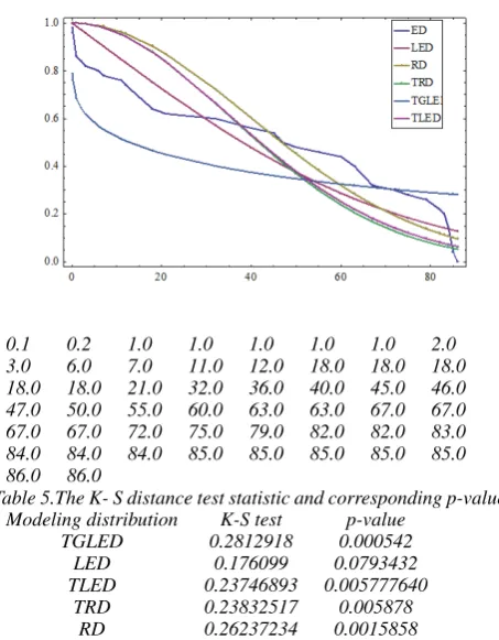
EXAMPLE 2. The lifetimes of 50 devices that were provided by (Aarset, 1987) are given in Table 4.

Table 4 Lifetimes of 50 devices.

0.1 0.2 1.0 1.0 1.0 1.0 1.0 2.0

3.0 6.0 7.0 11.0 12.0 18.0 18.0 18.0

[image:8.595.336.535.68.193.2]

18.0 18.0 21.0 32.0 36.0 40.0 45.0 46.0 47.0 50.0 55.0 60.0 63.0 63.0 67.0 67.0 67.0 67.0 72.0 75.0 79.0 82.0 82.0 83.0 84.0 84.0 84.0 85.0 85.0 85.0 85.0 85.0 86.0 86.0

Table 5.The K- S distance test statistic and corresponding p-values. Modeling distribution K-S test p-value

TGLED 0.2812918 0.000542

LED 0.176099 0.0793432

TLED 0.23746893 0.005777640

TRD 0.23832517 0.005878

RD 0.26237234 0.0015858

[image:8.595.320.547.373.664.2]

(9)

Fig. 5. Empirical and estimated survival functions of the LED, RD, TRD, TGLED and TLED models for (Leukemia data) Lifetimes of 40 patients suffering from Leukemia.

By calculating K-S test and corresponding p-values for TGLED and some special cases as LED, RD, TRD and TLED for men-tioned two survival data examples we can say that the distribution of TGLED can be appropriate to deal with Life data under different levels of significant. Table 3 and Table 5 contain some of the results that have been obtained for the two mentioned previous examples.

8. REFERENCES

1 Aarset, M.V.(1987). How to identify bathtub hazard rate. IEEE Transactions on Reliability R-36, 106 108.

2 Abouammoh, A., Abdulghani, S., Qamber, I.(1994). On partial orderings and testing of new better than renewal used classes. Reliability Engineering andSystem Safety 43, 37 41.

3 Aryal, G. R. and Tsokos, C. P.(2011). Transmuted Weibull distri-bution: A Generalization of the Weibull Probability Distribution. European Journal of Pure and Applied Mathematics, 4(2), 89-102.

4 Aryal. G. R. and Tsokos, C. P.(2009). On the transmuted extreme value distribution with applications. Nonlinear Analysis: Theory, Methods and applications, Vol. 71, 1401-1407.

5 Aryal, G. R. (2013). Transmuted Log-Logistic Distribution. J. Stat. Appl. Pro. 2, No. 1, 11-20.

6 Elbatal, I. ( 2013). Transmuted modified inverseWeibull Dis-tribution: AGeneralization of the Modified inverse Weibull Probability Distribution. International Journal of Mathematical Archive-4(8), 117-129.

7 Elbatal, I. and Aryal. G. R. .On the Transmuted AdditiveWeibull Distribution.Austrian Journal of Statistics (To Appear). 8 Lai, C.D., Xie, M., Murthy, D.N.P. (2001). Bathtub shaped

fail-ure rate distributions. In: Balakrishnan, N., Rao, C.R. (Eds.), Handbook in Reliability, vol. 20. 69 104.

9 Mahmoud, M.A.Wand Alam,F. (2010). The generalized linear exponential distribution, Statist. Probabil. Lett. 80 ,1005–1014. 10 Merovci, F.and Elbatal, I.( 2013). Transmuted

lindley-Geometric distribution and its applica-tions.Stat.ME.arXiv:1309:3774V1.(To submitted ).

11 Muhammad, K.S. and Robert, K.( 2013). Transmuted Modified Weibull Distribution: A Generalization of the Modified Weibull Probability Distribution. European Journal of Pure and Applied Mathematics. 6(1), 66-88.

12 Shaw,W. and Buckley,I. (2007).The alchemy of probability distributions: beyond Gram- Charlier expansions and a skew-kurtotic- normal distribution from a rank transmutation map. 13 Zhang,T , Xie, M,Tang,L and Ng,S (2005) Reliability and