HIGH LEVEL DESIGN FOR REAL TIME IMPLEMENTATION OF CSC ALGORITHM ON FPGA USING MATLAB & SIMULINK SIMULATION

(1)

ISSN: 1992-8645 www.jatit.org E-ISSN: 1817-3195

24

SOLVING A MULTI-DEPOT INVENTORY ROUTING

PROBLEM ARISING IN THE MOROCCAN FOOD MARKET

1

JAMAL LMARIOUH, 2DRISS BOUAMI, 3ANOUAR JAMALI, 4ABDESLAM MOZHER

1,2

QSM, Ecole Mohammadia d’Ingénieurs, Rabat, Morocco 1,3,4

CELOG, Ecole Supérieure des Industries du Textile et de l’Habillement, Casablanca, Morocco 4

MOAD, Ecole Mohammadia d’Ingénieurs, Rabat, Morocco

E-mail: [email protected], [email protected], [email protected],

4

[email protected]

ABSTRACT

In this paper, a real-life distribution problem faced by a Moroccan food company is solved. This problem is combining inventory and routing decisions. Vendor-managed inventory system is proposed to manage the company’s distribution. Transportation and inventory costs are simultaneously minimized which is known as the Inventory-Routing Problem (IRP). In our real-life problem, several plants deliver a set of customers with several types of products which can be defined as a multi-depot, multi-product and multi-vehicle IRP. A fleet of homogeneous vehicles is used to deserve customers and the inventory costs are paid at both the plant and at the customers. We propose a mixed integer linear program for this problem. Computational tests were carried out in four real-life instances which concern representative periods for the company. The results show the effectiveness of our approach.

Keywords: Inventory-Routing Problem; Vendor Managed Inventory; Depot; Vehicle;

Multi-Product

1. INTRODUCTION

In a changing world, companies must be agile to respond quickly to changes in market data. However, these changes do not always come from downstream, but they are also dangerous, of course, when they come from upstream. Companies must therefore be vigilant about the changes around them, upstream, downstream, internally and even in the political, social and regulatory environment. The changes that undergo our industrial partner came mainly from upstream. The declines in the cultivation of raw material as well as lower import prices have encouraged the trend of the company to import its raw material. The pace of the company’s various factories fell for the imported material through a single factory, that of Casablanca. The fixed costs of the plants became very important in relation to their production and consequently affect their profitability. Thus, a plant’s closure program was launched and the number of plants decreases from 14 to 5. The closure of several plants has changed significantly the company’s distribution pattern. Indeed, much of the flow passing through the plant of Casablanca, which has completely changed the company’s distribution program. Thus,

in order to maximize service level and minimize costs while avoiding stockouts and overstock, we propose to use Vendor Managed Inventory (VMI) and to solve the problem as a depot, Multi-product, and Multi-vehicle Inventory Routing Problem (3MIRP).

Recently, the Moroccan government eliminated progressively its subsidies on the price of fuel,

indeed transportation costs have increased

significantly. Companies, in order to find a good tradeoff between service level and costs, must

minimize simultaneously transportation and

inventory costs while avoiding stockouts and overstocks.

In this paper, we discuss a case study of a Moroccan food company. Our industrial partner deals with a total of five different types of products produced by five plants. Each plant produces one, many or all products and owns a local warehouse.

(2)

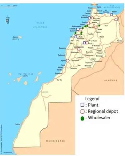
25 the plants and all customers are shown on the following map of Morocco (Figure 1).

[image:2.612.91.291.239.490.2]

The transportation cost has increased significantly last years, since a large quantity of pallets have to be transported from the plant of Casablanca caused by the closure of several other plants, Indeed many customers are now served from the farthest Casablanca plant instead of the nearest closed plants. This has led the company to create and develop new contracts with transporters which state that the company charters trucks according to its need and pay them for the distance travelled.

Figure 1: Map Of Morocco And Location Of The Plants And Customers (Source: Routard (November 2015))

Production levels are supposed constant and are not subject to operational changes. The distribution planning is done manually based on the experience of planners that take into account demand forecasts and inventory levels at customers. However, as there are several plants, several products and the plants don’t produce necessary all products, the planner find difficulty to plan the distribution in an optimal way to avoid stockouts and overstock and minimize the total logistic cost. Indeed the company must review its planning approach to achieve these goals.

Our problem can be defined as a rich 3MIRP. The IRP has been formally introduced more than 30 years ago by [5], many practical and technical contributions have been followed. For a recent review of IRPs, see [12]. In what follows we review the most relevant to our case.

The single product IRP was studied in many papers ([3], [8], [10] and [11]) and the case with several products is recent and significantly more difficult. Reference [24] has developed a hybrid

genetic algorithm, a two-phase variable

neighborhood search was developed by [22] and [23], and reference [17] has proposed an ant colony optimization algorithm. For exact algorithms, reference [9] has developed an exact branch- and-cut algorithm. The multi-depot case was treated by [28], they proposed a mixed integer linear program to solve it. Reference [30] solved the multi-depot IRP using a decomposition and coordination method, they use a genetic algorithm to design the coordination values and an adaptive adjustment scheme for the routes.

Maritime industry was the sector in which many real-life applications were developed ([4], [6], [7], [13], [16], [25], [31] and [32]). Maritime applications are relevant to our case because they also have a many to many structure, but their application is very different from the case of multi-depot IRP. Non-maritime applications include the transportation of gases by tanker trucks ([5]), the

automobile components industry ([1]), the

distribution of perishable products ([14] and [15]), fuel delivery ([26])) and the distribution of grocery and food products ([15], [18], [19], [20] and [21]). A review of practical applications can be found in [2].

The main contribution of this paper is to solve a real-life and rich 3MIRP arising in the food industry in Morocco. We treat the multi-depot case which is not very explored in the literature. We are then capable of proposing high quality solutions to our partner, which significantly outperforms their current solutions.

The remainder of the paper is organized as follows. In Section 2, we describe the problem and propose an integer linear programming formulation for it. In Section 3, we present computational experiments followed by conclusions in Section 4.

2. ROBLEM DESCRIPTION AND

FORMULATION

In order to formulate the problem by means of an integer linear programming model we

define it on an undirected graph G={W,ε}, where W

= U ∪ V’ is the vertex set and ε={(i,j),i<j} is the

edge set. U={1,…,l} represents the set of plants

(depots) and V’={1,…,n} represent the set of

customers which are partitioned as regional depots

(3)

26

depot and customers. Each plant u ∈ U and

customer i ∈ V’ incurs respectively inventory

holding cost and per period, and has an

inventory capacity and respectively. The

company distributes a set M={1,…,M} of products,

which are all measured in terms of number of

pallets. The length of the planning horizon is p,

measured in discrete time periods t ∈ T={1,...,p}.

The quantity of product m made available at the

plant u in period t is . The inventories are not

allowed to exceed the holding capacity and cannot be negative. At the beginning of the planning horizon the decision maker knows the current

inventory level of each product m at each plant

u and at each customer i, and receives the

information on the demand of each location i

for each product m and period t. We assume that the

quantities received by location i of product m

from plant u with vehicle k in period t can be used

to meet its demand in that period. An unlimited

fleet of vehicles K is available. We then identify

each vehicle k ∈ K={1,...,K }, each with capacity Q

(in number of pallets). A routing cost is

associated with edge (i,j) ∈ ε in the route of plant u

∈ U. The objective of the problem is to minimize

the total routing and inventory holding costs while avoiding stockouts and overstock and meeting the demands for each product at each location in each period.

The following decision variables are used by model. Integer undirected routing variables

are equal to the number of times that edge (i, j) ∈

ε

is used on the route of vehicle k coming from plant

u in period t; binary variables are equal to one

if and only if location i ∈ V is visited by vehicle k

coming from plant u in period t; integer variables

represent the inventory level of product m at the plant u at the end of period t; integer variables

represent the inventory level of product m at a

customer i at the end of period t; integer variables represent the quantity of product m delivered to location i by vehicle k coming from plant u in

period t. The problem can then be formulated as

follows:

Subject to

The objective function (1) minimizes the total inventory and routing costs. Constraints (2) and (3) define inventory conservation at the plants and the customers respectively. Constraints (4), (5) and (6) impose maximal inventory level at the plants and the customers. Constraints (7) link the quantities delivered to the routing variables. In particular, they only allow a vehicle to deliver any products to a customer if the customer is visited by this vehicle. Constraints (8) ensure the vehicle capacities are respected. Constraints (9) and (10) are degree constraints and subtour elimination constraints, respectively. Constraints (11) − (16) enforce integrality and non-negativity conditions on the variables.

(4)

27 Constraints (17) and (18) are referred to as logical inequalities. They enforce the condition that if the supplier is the successor of a customer in the route of vehicle k coming from plant u in period t, i.e., = 1 or 2, then i must be visited by the same

vehicle, i.e., = 1. A similar reasoning is applied

to customer j in inequalities (18). Constraints (19)

include the supplier in the route of vehicle k coming

from plant u at the period t if any customer is

visited by that vehicle in that period. Constraints (20) ensure that customer i is visited at least the number of times corresponding to the right-hand side of the inequality. This inequality is only valid if the fleet is homogeneous. It was originally developed for the single-vehicle case by [3] and was later extended to the multi-vehicle case by [9].

3. PROBLEM DESCRIPTION AND FORMULATION

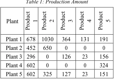
[image:4.612.100.291.480.613.2]

Our industrial partner owns five plants producing five types of products as shown in table 1.

Table 1: Production Amount

Plant

P

ro

d

u

ct

1

P

ro

d

u

ct

2

P

ro

d

u

ct

3

P

ro

d

u

ct

4

P

ro

d

u

ct

5

Plant 1 678 1030 364 131 191

Plant 2 452 650 0 0 0

Plant 3 296 0 126 23 156

Plant 4 602 0 0 0 324

Plant 5 602 325 127 23 151

Once production is finished, products are stored at the plant’s warehouses. The holding cost of a pallet at the plants is on average about 2.5 MAD (Moroccan Dirham) per day. Products are shipped to a set of customers that are divided in two groups. The first one contains 8 regional depots belonging to the company, with an average daily inventory holding cost of 2.7 MAD per pallet. The second group consists of 7 wholesalers of which the

company does not pay the inventory holding costs.

We consider a maximal number of 27

homogeneous vehicles with a capacity of 24 homogenous pallets.

We perform different computational

experiments on real-life based instances. Studying the flow of the company, we have identified four principal periods in which the distribution flow change considerably. In each month, the demand changes considerably if we are in the three first weeks or we are in the last week. Indeed in the last week of each month, the demand arises in comparison with other weeks. The second observation is that in each week there are two periods. In the first three days, the demand is lower than in the second three days (we consider a week of 6 days as the company doesn’t work Sundays). In conclusion, we have used four instances for our computational tests corresponding to the four cases explained below. Instances of the three first days of a normal week are called L. Instances of the three second days of a normal week are called M. Instances of the three first days of the last week of the month are called H and instances of the three second days of the last week of the month are called V.

The strategy of our partner to find solutions consists to ship a full-truck load (FTL) to any customer whose associated demand cannot be satisfied from the stock. To avoid situations in which the Casablanca plant exceeds its own inventory, the planner must ship extra product amounts in FTL to regional depots while ensuring that their storage capacities are sufficient to enable their reception.

The planner of the company must decide on the quantity to be delivered by commodity from each plant and to each customer, this is very complex to do manually. Thus, stockouts and overstocks occur in factories or among customers. What is even more expensive is that customer orders cannot be fulfilled whereas products are available in sufficient quantity, but they were sent to the wrong place.

(5)

[image:5.612.89.295.134.226.2]

28 continuously correct the schedule of the next three days.

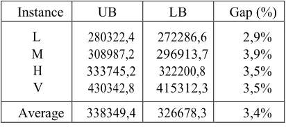
Table 2: Assessment Of The Performance

We present in Table 2 the associated results. We note that in the totality of cases, the GAP is reasonable with an average about 3,4 %. The total cost increases from L to V which is quite logical.

We have decomposed the total cost into its transportation and inventory holding components. These figures are shown in Table 3. We note that in going from L to V, the percentage of inventory costs decreased comparing to transportation costs, this is explained by the fact that for low instances, the quantities transported are smaller which creates larger inventories since the production is constant.

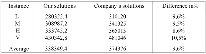
Finally, we compare our solutions with those currently employed by our industrial partner. This comparison is presented in Table 4. It should be noted that it is difficult to have accurate business solutions. We estimated these solutions based on our understanding of the business organization and the method used by the planner, we however based on the most favorable case for the company. We note that for all instances, our approach performs better than one proposed by the company by up to 10.5%. The advantage of our approach lies also in the fact that it eliminates stockouts and overstocks while allowing visibility and ease of planning.

3. CONCLUSION

We have presented a complex real-life problem arising in Moroccan food market. Several plants have to deliver different types of products to a set of customers. Our goal was to minimize the sum of transportation and inventory costs while avoiding stockouts and overstocks both at plants and customers. We have presented an integer formulation which we developed to our specific context. The results indicate that our approach outperforms the company one for all instances.

REFRENCES:

[1] J. Alegre, M. Laguna, and J. Pacheco,

“Optimizing the periodic pick-up of raw materials for a manufacturer of auto parts”

European Journal of Operational Research, 179(3):736–746, 2007 .

[2] H. Andersson, A. Hoff, M. Christiansen, G.

Hasle, and A. Løkketangen, “Industrial aspects and literature survey: Combined inventory

management and routing” Computers &

Operations Research, 37(9):1515–1536, 2010.

[3] C. Archetti, L. Bertazzi, G. Laporte, and M. G.

Speranza, “A branch-and-cut algorithm for a vendor-managed inventory-routing problem”

Transportation Science, 41(3):382–391, 2007.

[4] D. Bausch, G. Brown, and D. Ronen,

“Scheduling short-term marine transport of

bulk products” Maritime Policy &

Management, 25(4):335–348, 1998.

[5] W. J. Bell, L. M. Dalberto, M. L. Fisher, A. J.

Greenfield, R. Jaikumar, P. Kedia, R. G. Mack, and P. J. Prutzman, “Improving the distribution

of industrial gases with an on-line

computerized routing and scheduling

optimizer” Interfaces, 13(6):4–23, 1983.

[6] L. Bertazzi, G. Paletta, and M. G. Speranza,

“Deterministic order-up-to level policies in an

inventory routing problem” Transportation

Science, 36(1): 119–132, 2002.

[7] M. Christiansen, K. Fagerholt, T. Flatberg, O.

Haugen, O. Kloster, and E. H. Lund, “Maritime inventory routing with multiple products: A case study from the cement industry”

European Journal of Operational Research, 208 (1):86–94, 2011.

[8] L. C. Coelho and G. Laporte, “The exact

solution of several classes of inventory-routing

problems” Computers & Operations Research,

40(2):558– 565 2013a.

[9] L. C. Coelho and G. Laporte, “A

branch-and-cut algorithm for the product

multi-vehicle inventory-routing problem”

International Journal of Production Research, 51(23–24):7156–7169, 2013b.

[10]L. C. Coelho, J.-F. Cordeau, and G. Laporte,

“Consistency in multi-vehicle

inventory-routing” Operations Research Part C:

Emerging Technologies, 24(1):270–287,

2012a.

“The inventory-routing problem with

transshipment” Computers & Operations

Research, 39(11):2537–2548, 2012b.

Instance UB LB Gap (%)

L M H V

280322,4 308987,2 333745,2 430342,8

272286,6 296913,7 322200,8 415312,3

2,9% 3,9% 3,5% 3,5%

(6)

29

“Thirty years of inventory- routing”

Transportation Science, 48(1):1–19, 2014.

[13]F. G. Engineer, K. C. Furman, G. L.

Nemhauser, M. W. P. Savelsbergh, and J.-H. Song, “A branch-and-price-and-cut algorithm for single-product maritime inventory routing”

[14]A. Federgruen and P. H. Zipkin, “A combined

vehicle-routing and inventory allocation

problem” Operations Research, 32(5):1019–

1037, 1984.

[15]A. Federgruen, G. Prastacos, and P. H. Zipkin,

“An allocation and distribution model for

perishable products” Operations Research,

34(1):75–82, 1986.

[16]R. Grønhaug, M. Christiansen, G. Desaulniers,

and J. Desrosiers, “A branch- and-price method for a liquefied natural gas inventory routing

problem” Transportation Science, 44(3):400–

415, 2010.

[17]S.-H. Huang and P.-C. Lin, “A modified ant

colony optimization algorithm for multi-item inventory routing problems with demand

uncertainty” Transportation Research Part E:

Logistics and Transportation Review, 46(5): 598–611, 2010.

[18]H.-S. Hwang, “A food distribution model for

famine relief” Computers & Industrial

Engineering, 37(1):335–338, 1999.

[19]R. Lahyani, L. C. Coelho, M. Khemakhem, G.

Laporte, and F. Semet, “A multi-compartment vehicle routing problem arising in the

collection of olive oil in Tunisia” Omega,

51(1):1–10, 2015.

[20]S.-C. Liu and J.-R. Chen, “A heuristic method

for the inventory routing and pricing problem

in a supply chain” Expert Systems with

Applications, 38 (3):1447–1456, 2011.

[21]M. Mateo, E.-H. Aghezzaf, and P. Vinyes, “A

combined inventory routing and game theory approach to solve a real-life distribution

problem” International Journal of Business

Performance and Supply Chain Modelling, 4 (1):75–89, 2012.

[22]A. Mjirda, B. Jarboui, R. Macedo, and S.

Hanafi, “A variable neighborhood search for the multi-product inventory routing problem”

Electronic Notes in Discrete Mathematics, 39(1):91–98, 2012.

[23]A. Mjirda, B. Jarboui, R. Macedo, S. Hanafi,

and N. Mladenović “A two phase variable neighborhood search for the multi-product

inventory routing problem” Computers &

[24]N. H. Moin, S. Salhi, and N. A. B. Aziz, “An

efficient hybrid genetic algorithm for the

multi-product multi-period inventory routing

problem” International Journal of Production

Economics, 133(1):334–343, 2011.

[25]J. A. Persson and M. Gothe-Lundgren,

“Shipment planning at oil refineries using column generation and valid inequalities”

European Journal of Operational Research, 163(3):631–652, 2005.

[26]D. Popović, M. Vidović, and G. Radivojević,

“Variable neighborhood search heuristic for the inventory routing problem in fuel delivery”

Expert Systems with Applications, 39

(18):13390–13398, 2012.

[27]W. W. Qu, J. H. Bookbinder and P. Iyogun,

“An integrated inventory-transportation system with modified periodic policy for multiple

products” European Journal of Operational

Research, 115(2):254–269, 1999.

[28]N. Ramkumar, P. Subramanian, T. Narendran,

and K. Ganesh, “Mixed integer linear programming model for multi-commodity

multi-depot inventory routing problem”

OPSEARCH, 49(4):413,429, 2012.

[29]D. Ronen, “Marine inventory routing:

shipments planning” Journal of the

Operational Research Society, 53(1):108–114, 2002.

[30]L. Shan-zuo and W. Yao-hua, “Solving

multi-depot inventory-routing problems based on decomposition and coordination method”

Journal of Highway and Transportation Research and Development, 9:035, 2007.

[31]M. Stålhane, J. G. Rakke, C. R. Moe, H.

Andersson, M. Christiansen, and K. Fagerholt, “A construction and improvement heuristic for a liquefied natural gas inventory routing

problem,” Computers & Industrial

Engineering, 62(1):245–255, 2012.

[32]K. T. Uggen, M. Fodstad, and V. S. Nørstebø,

“Using and extending fix-and- relax to solve

maritime inventory routing problems” TOP,

(7)

[image:7.612.98.513.115.208.2]

30

Table 3: Decomposition Of The Total Cost

Table 4: Comparison With The Company’s Solutions

Instance Total cost Transportation cost (In %) Inventory cost (In %)

L M H V

280322,4 308987,2 333745,2 430342,8

161664,4 190096,4 214722,4 310530,4

57,7% 61,5% 64,3% 72,2%

118658,0 118890,8 119022,8 119812,4

42,3% 38,5% 35,7% 27,8%

Average 338349,4 219253,4 63,9% 119096,0 36,1%

Instance Our solutions Company’s solutions Difference in%

L M

H V

280322,4 308987,2 333745,2 430342,8

310120 341325 365013 481046

9,6% 9,5% 8,6% 10,5%

[image:7.612.131.481.241.333.2]