GLOBAL PATH PLANNING BASED ON SKELETON
EXTRACTION ALGORITHM
JUN WANG, MING LI, DONG LI
School of Information and Electrical Engineering, China University of Mining and Technology,
Xuzhou 221116, Jiangsu, China
ABSTRACT
Skeleton extraction algorithm can transform two-dimensional map into a skeleton diagram, which provide more convenience to global path planning of the complex map. This article first extracts skeleton extraction of the global map using the skeleton extraction algorithm and finds all paths of flat map. Based on this we can use search algorithms to search, and find a feasible path connecting starting point and target point. At last we use the optimized algorithm to find optimize the path to achieve the global path planning and optimization in the map. In the simulation, we use the complex maze of the map to validate the algorithm and the effect of it in simulation condition show the effectiveness of the algorithm.
Keywords: Skeleton Extraction, Global Path Planning, A* Algorithm, PSO, Particle Filter, Map Creating
1. INTRODUCTION
The traditional path planning method is planned without suggested path, so it meets the problems above [1, 2]. Due to path planning, usually global map is known, and there is unknown barrier only in part of map. If we can get suggested path according to global path, and then implement optimization algorithm based on suggested path, we will get the optimal route.
According to this idea, this article finds all paths of global map using the skeleton extraction algorithm. On this basis we can find a path connecting starting point and target point and optimize it. Thus we achieve the global path planning and optimization in complex map.
2. SKELETON EXTRACTION
ALGORITHM TO GENERATE GLOBAL PATH
In two-dimensional map the robot’s searching space is very large, so it is difficult to find a feasible path. If the map can be transformed into one-dimensional, the search will become simple, and it will get the result. Skeleton extraction algorithm can transform two-dimensional planar map into one-dimensional road map, which is to extract the skeleton plane of planar map. The method broke through the difficulties to recommend path to plan path, and solved the key issues of complex two-dimensional map.
1
4
2
5
3
6
[image:1.612.372.477.356.460.2]7
8
9
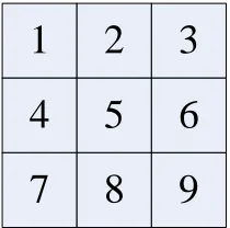
Figure 1:The Basic Filter Unit
Figure 1 shows the basic filter unit in the skeleton extraction algorithm and the No.5 pixel is the real point which need to corrode.
Using such a basic unit can examine the surroundings of the No.5 pixel, and by the
information we can determine the 5 pixels to be eroded or stayed. By the filter in Figure 1, each feasible pixel in one-color map is filtered, although it is impossible to process pixels in outermost ring, the feasible path cannot be in sideline. Therefore, the filter is started from penultimate layer. That is the pixels in outermost layer are infeasible points. The process of skeleton extraction is like this:
1. for each feasible point in the outermost lap.
2. If center point of filter convex point && whether feasible points are connected is not influenced by removing the center point of filter.
4. Else center point of filter remains its value.
5. End For.
6. Update feasible points in map.
7. If the number of feasible in map equals that last time.
8. Then END.
9. Else go to STEP 1.
3. A*ALGORITHM TO SEARCH A
FEASIBLE PATH
Getting a map of the skeleton, as long as connecting the starting point and destination point to the nearest path, the starting points and destination points can be connected. Then we need to select an optimum feasible path connecting the starting points and destination points as the recommended path. Then using the optimization algorithm to optimize the recommended path ,thus to get the optimal path of the robot .There are many ways to search the feasible path connecting the starting points and destination points, such as breadth-first search, depth first search, bounded depth-first search, etc. They all belong to the blind search methods and are used to solve the smaller problems. Blind search is the search strategy in accordance with pre-set strategy, and the useful information in search process is not used to improve policy. Thus the search process is less efficient [3], and wastes a lot of space and time resources, which is not conducive to solve the larger problem. A more efficient search method is heuristic search, which uses heuristic information that is the related information about problem solving. This information will prompt to search towards a more possible path and avoid detours. In the expansion nodes, the heuristic information will usually compare with all the extended nodes and identify the nodes which are more likely to search [4]. So we only need to search part of the space of all paths and the method is efficient.
In heuristic search, how to examine the importance of the nodes, and how to determine heuristic information and select the more important nodes are the key problems of heuristic search. Feasible paths are relatively simple, and using A * algorithm can quickly find the goal, so we can use the A * algorithm to find the optimal path. Existing cost function g is calculated with the sum of traversed grids and the predicted cost function h is calculated with the distance from node to the target point. Getting from the skeleton extraction algorithm is the skeleton which is a map with a
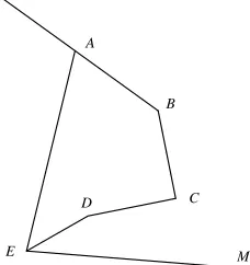
ring, so the first problem of undoing ring is to solve in the search algorithm. Figure 2 shows A * algorithm schematic diagram of ring solutions:
B
D
E M
[image:2.612.365.479.137.258.2]C A
Figure 2:A * Algorithm Schematic Diagram Of Ring
When searching point A, comparing the point B and point E, then choose one of them to go forward. It needs to calculate the cost f of point B point and E, which costs f are the sum of their existing costs g and expected costs h. Existing costs can be expressed as the number of routes through the grid, and this value can be calculated with the sum of existing costs of point A and point A to point B or point E of the grid. And their expected costs are calculated by the containing points through their straight-line distance from the target point. Assuming the point M as the target point, then we can clearly see that the cost of point B is less than that of point E. Therefore, A* search algorithm select B point to go forward, and point E will be credited to OPEN table. When the algorithm starts from the point B and passes through point C and point D, then backs to point E, the cost of this route ABCDE has cost higher than the AE. So we can solute ring at point E. At this point ABCD becomes a twig, and AE becomes another one. The algorithm reaches the target point through AE.
4. PARTICLE SWARM OPTIMIZATING
PATH
However, PSO can get others' to offset its own weaknesses, and can develop their own advantages [6, 7]. So the convergence speed of PSO algorithm is faster than genetic algorithms. Based on these advantages of Particle Swarm Optimization, and combining with high real-time path planning requirements, we can select PSO algorithm to optimize the path.
In this article, applying the particle swarm algorithm to the whole path and vibration all the paths is unrealistic. Before PSO we should carry out the second iteration and the third iteration, so and let the path becomes one by one small line that satisfies certain conditions. If after the second iteration, the path connected end to end is not obstructed, then it will be connected directly. If the barriers do not exceed 3, apply the particle swarm algorithm to optimize. If the path is more than 3, then continue to carry out the second iteration and the third iteration until meeting the application of PSO or it can be directly connected. Application of the second and third iteration is to make all the points can be optimized. Figure 3 shows the local particle swarm optimization model with only two obstacles.
X
Y
1 2
3 4
[image:3.612.359.480.208.430.2]5
Figure 3:Mode Of Particle Swarm Path Optimization
Black thick lines in Figure indicates the walls and other obstacles, and fine line stands for the path found by the skeleton algorithm and search algorithm, which is the path needed to optimize. In Figure 3, this path acts as a particle. As the calculation of particle swarm optimization is faster, the number of particles can be taken relatively large, equivalent to a lot of jump path. Dimension of particle swarm has heavy influence on the convergence rate of PSO. If the dimension of particle swarm is too large, The PSO is difficult to weaken [8]. Dots on line in Figure 3 represent components of each dimension of particles. Particle's velocity is represented by a vector. Particle velocity in each dimension vertical direction of the connection is described by the previous one-dimensional position and the latter one-dimensional position. Particles shown in Figure 3, its 3-dimensional velocity direction is vertical to
the connection of 2-dimensional state and 4-dimensional state.
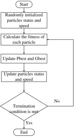
The next key issue is to determine the objective function, which is created according to specific issues. In this article, if you want to achieve the effect of optimal path, the objective function is the length of the path. In the grid map, the length is described by the number of grid. Figure 4 shows the flow chart of particle swarm optimization.
Start
Randomly initialized particles status and
speed
Calculate the fitness of each particle
Update Pbest and Gbest
Update particles status and speed
Termination condition is met
End
No
Yes
Figure 4 Flow Chart Of Particle Swarm Optimization
5. PARTICLE FILTER LOCALIZATION
ALGORITHM
On the basis of global path planning, in order to apply the robot to walk along a predefined optimized route, the robot requires self-located. It is necessary to use particle filter, which can eliminate detection error and other errors in the robot probability movement model and locate a robot.
Particle filter algorithm is an approach using the idea of probability theory to calculate the robot state, which avoids the dependence of the most likely event and uses all the circumstances’ probability distribution that may arise to describe the information [9]. So that it can describe obscurity and credibility in a reliable mathematical way and enable it to adapt to all the uncertainty [10].
[ ] [ ] 1
[ ] [ ]
[ ] [ ]
1
_ _ mod ( , );
_ mod ( , );
, ;
1
to the probability pro
t t
m m
t t t
m m
t t t
m m
t t t t
X X
for m to M do
x sample motion el u x
measurement el z x
X X x
dedfor
for m to M do
ω
ω
−
= = Φ
= =
=
= + < >
=
[ ]
[ ] [ ]
portional to extract particle i
from the ;
, ;
m t
t
m m
t t t t
X
X X x
endfor
ω
ω
= + < >
Sample_motion_model ( ut , [ ]
1 m t
x− ) said that according to the particles’ movement model of t-1 time we can get a sample of the state probability prior distribution at the time. Measurement model (zt,
[ ]m t
x ) said that according to the observation model of the particle m we can observe the
probability of observation informationzt.
In the particle filter algorithm, the number of particles is the most direct factor of computing resource consumption. The more particles, the computation is larger. When the number is small, the particles is very easy to fall into other farther states away from the true solution, which lead the true position and orientation searching becoming extremely difficult[11,12]. In theory, the number of particles is as large as possible. Because when the particle number is large enough, they will be sufficiently close to the true posterior probability distribution. If the number of particles is M, then
the probability of error is 1
O M
=
.However, the
increase of the number of particles will lead to the increase of computation. Therefore, the number of particles should be selected according to the requirements of the actual precision.
In addition, the comparison of the similarity between observed information and particle measurement information is the most important factor when calculating particle weights. The relationship is as follows:
[ ]m ( | [ ]m ) t p zt xt
ω =η (1)
Ŋ is the right of a parameter renormalization, and
t
z is particle observation position. ( | [ ]m)
t t
p z x is
the probability of observing observed position based on the particlext[ ]m .
Euclidean distance used here to express this similarity. 2 1 ( , ) ( ) M i i
real particle real particle i
D X X X X
=
=
∑
−(2)
M is the particle’s column number. Then
according to the actual simulation results the weight
i
ω formula can be adjusted to:
4
1
( , ) 1
i
real particle
D X X
ω =
+ (3)
The range of ωi is (0~1). Weight normalization
can be carried out in accordance with the following algorithm.
lg ormalize_Weight()
0
for 1 to M
total total
end for
for 1 to M
/
end for return
i
i i
A orithm N double total i i total ω ω ω = = = + = =
The weight of each particle of particle concentration divides the weight of all particles and which can be as the weight of the particles.
6. CREATE AND UPDATE MAPS
When the robot moves in the predetermined route using particle filter, it is probable to encounter some obstacles which are in the pre-set a good route and prevented the robot to move forward. In order to avoid these obstacles, skeleton extraction algorithms need to be used for real-time planning capabilities. The required information is the latest map information, so creating and updating maps is essential for the whole process. Here the map update and creation are executed by the Monte Carlo algorithm. It constantly calculate the probability of the grid map, then uses gray to indicate the probability in the grid map.
6.1Update Grid Map
local maps; second, according to the expected path generated by the particle filter update the relative position where local map previously observed all times in the global map.
For the first aspect of the update, we select the learning style of the probability regeneration. In order to make it easy to indicate the probability of each grid, we use P to indicate the probability
[ ij 0]
P S = occupied by the grid.
That is pt = pt−1+α(pv−pt−1)* |pv−0.5 |
t
p : The probability of occupied grid at t time;
1 t
p− : The probability of occupied grid at t-1
time;
v
p : An estimated probability from the laser
range finder data at t time;
α : learning coefficient:α <<1.
The significance of this type has the following:
(1) |pv−0.5 |the significance is to determine the
changing credibility in the grid;
(2) pv−pt−1 the purpose is to determine the
credibility of the grid to increase or decrease;
(3) αLearning coefficient, its significance is to decide the learning rate.
The most important problem is how to get the estimated probability in the formula. We cannot use the exact formula to describe the probability
distribution of robot pose
x y θ
. Usual solution is to
use the Monte Carlo method to obtain approximately the probability distribution.
For the second aspect of the update, after resembling particle filter particles in the algorithm will change accordingly and the map relative position created by robot moving path in front will change. In order to create more accurate maps, we re-adjust the relative positions where the local environment information previously observed by laser range finder in the global map and get the latest global map.
6.2 The Probability Map Creation Based On Monte Carlo Method
In the part of map update, from updating formula for the probability of grid, we can know how to get
estimated probability pv of the grid after each
measurement is a key issue. Thus the algorithm proposed to approximate pvusing the principle of Monte Carlo sampling.
To describe the algorithm easily, map the
location of the grid indicated
bym iij( ∈[0, ],m j∈[0, ])n . The data observed by
laser range finder recorded asz0:t:{ , ,z z z0 1 2,..., }zt .
Robot pose is denoted by x0:t :{ ,x x x0 1, 2,..., }xt .
Each time have L particles {xt0,xt1,xt2,...,xtl} . Probability of updated global maps isp m( ij|x0:t,z0:t). The estimated probability of each
grid based on observations is (p mij|x zt, )t . As we adopt the Monte Carlo, we abridge name of the algorithm as MCM. The algorithm is as follows.
MCM
( (
p m
ij|
x
0:t,
z
0:t),
x
0:t,
z
0:t)
For k=1 to K do
Sample
ξ
k~
p
(
x
t)
For each grid cell
m
ij do)
,
|
(
m
ij kz
tp
ξ
By laser_probability_modelEnd for
1
(
ij|
t, )
t(
ij|
t, )
t(
ij|
k, )
tp m
x z
p m
x z
p m
z
k
ξ
=
+
End for)
5
.
0
)
,
|
(
(
|
)
,
|
(
)
,
|
(
|
)
,
|
(
)
,
|
(
1 ; 0 1 : 0 1 1 ; 0 : 0−
×
−
+
=
− − − − t t ij t t ij t t ij t t ij t t ijz
x
m
p
z
x
m
p
z
x
m
p
z
x
m
p
z
x
m
p
α
Return
p m
(
ij|
x
0:t,
z
0:t)
The core idea of this algorithm is using Monte
Carlo method to approximate the robot pose
x
y
θ
error distribution to get the estimated probability(
ij|
t, )
tThrough the experiment, the grid map getting from the algorithms is shown in Figure 5.
[image:6.612.127.278.135.286.2]
Figure 5 The Creation Of The Grid Map
The color depth of each grid map indicates the probability of its occupied. The points are darker, the occupied probability is greater. From the experimental results, the algorithm has good adaptability to environment. The algorithm has high accuracy to process laser range finder information. The space in physical environment can be expressed well. We can see from the algorithm model, this advantage comes from:
(1)Algorithm takes serious repercussions created by robot pose error to the map generated in the moving process into account ;
(2)The model of laser range finder established by this method is based on historical probability information to obtain the final state of grid cells. This method improves the reliability of interpretation to the space environment.
7. SIMULATION
7.1 Simulation Platform and Structure
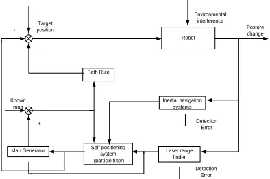
Figure 6 shows the block diagram of the control system simulation platform, in which the input information including the known map, location of target , detection signal by inertial navigation systems and laser range finder on the posture change and the actual environment. Interference information is produced by the detection error of inertial navigation and the laser range finder and the interference of external environment on the robot, including the promotion error, etc. System output is pose changes of the robot and improvement on the known map by the map generator that is map building. Firstly system plans paths with the known maps, connecting the starting position and the
destination to create a feasible path. Then the particle filter does Self-localization combined with the data detected by inertial navigation systems and laser range finder, the robot being always walking on the planned path. Pose changes produced on the process are used to control the motor of the robot, of course, controlling the robot's walking in the simulation environment. In addition the particle filter self-position system is also used to serve the map generator. Precisely positioning makes the map generator to use the laser range finder to obtain updating map data and creating map. When the robot moves to the target location, the map generator has completed its work creating a latest global map, achieving the purpose of inspection.
Path Rule
Robot
Map Generator
Inertial navigation systems
Self-positioning system (particle filter)
Laser range finder Target
position
Environmental interference
Posture change
Detection Error
Detection Error Known
map
-+
+
Figure 6 The Algorithm Flow Chart
7.2 Algorithm Flow
[image:6.612.319.516.279.410.2]Known map
Skeleton extraction
A * search algorithm
Particle Swarm Optimization
Particle Filter
Map Generation Algorithm
Walking routes in the original planning
Reach the destination
End N
Y N
Y
[image:7.612.87.522.61.676.2]Latest Global Map Start
Figure 7 The Algorithm Flow Chart
[image:7.612.97.309.68.466.2]7.3 Experimental results
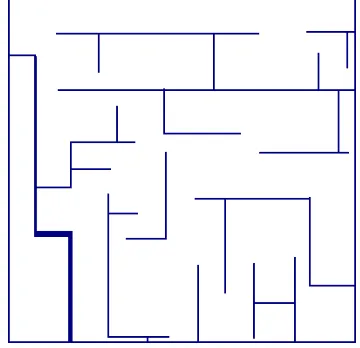
Figure 8 is the simulation effect drawing of skeleton algorithm for global path planning.
A
B
C
D
Figure 8 Path Planning
[image:7.612.109.289.544.718.2]algorithm to search the path in Figure (B). The full line in Figure (D) is the optimal path, the dotted line is not optimal. It can be seen from the figure that skeleton extraction algorithm, A * search algorithm and particle swarm optimization algorithm are very effective to plan path. The algorithm can still be a good solution to planning problems, in such a complex mazy map. Figure 9 describes the simulation effect of global map.
A
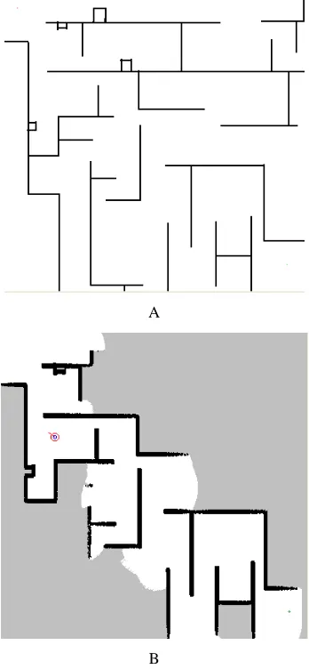
[image:8.612.113.287.208.584.2]B Figure 9 Real-Time Path Planning
Figure A is the actual map while figure B is created in real-time. In Figure B, the gray areas cannot be detected by the robot, and the black are the detected walls. The big red circle on behalf of the robot, the small blue circle on behalf of the localization result by particle filter, the figure shows particle filter positioning is quite accurate based on the global path planning and it can converge to the true pose of the robot. Map building can also create a map in real-time, and it provides sufficient information to the skeleton extraction
algorithm to ensure that the robot reaches the target successfully.
8. CONCLUSION
In this paper, it uses skeleton extraction algorithm for processing two-dimensional map to get the skeleton of the plane map, then uses A * algorithm to find paths connecting starting point and destination point, finally uses particle swarm algorithm to optimize the paths to find the optimal initial route for the robot. Simulation results also verify the effectiveness of the algorithm which can solve complex map of the route planning and optimization problems. In this paper, based on the path planning, it is proposed to use the particle filter algorithm to make the robot self-positioning and create and update maps in real time. At the same time, the map information is provided to the skeleton extraction algorithm making it can create real-time route when the robot encounters obstacles in planning routes. These series of interconnected algorithm together ensures the normal operation of the robot.
Of course there are still many issues to be discussed. Optimizing the path after the search does not guarantee the final result is optimal, because the path not being selected in the selection algorithm may be more optimized well. This problem can be solved by determining the number of extreme points according to the number of independent obstacles in the map. If the number of independent obstacles is n, then there should be 2n extreme points. When the extreme point is small, the optimal solution can be found by simple algorithm such as mountain climbing; when there are many extreme point s, the problem can be solved by genetic or the particle swarm algorithm and so on. These problems have yet to be studied further.
ACKNOWLEDGEMENTS
REFERENCES:
[1] Lee MJ, Hwang GH, “Object tracking for mobile robot based on intelligent method”, Artif Life Robotics, Vol. 13, No.1, 2008, pp.359-363. [2] Burgard W, Moors M, “Coordinated multi-robot
exploration”, IEEE Trans Robotics, Vol.21, No.3, 2005, pp.376-386.
[3] Fu YY, Wu CJ, “A time-scaling method for near time-optimal control of an Omni-directional robot along specified paths”, Artif Life Robotics, Vol. 13, No.1, 2008, pp.350-354.
[4] Guzzoni D, “Many robots make short work”, AI Mag, Vol. 18, No.1, 2006, pp.55-64.
[5] Belkhouche F, “Reactive path planning in a dynamic environment”, IEEE Trans Robotics, Vol. 25, No.4, 2009, pp.902-911.
[6] Ferguson D, Howard TM, Likhachev M, “Motion planning in urban environments”, J Field Robotics, Vol. 25, No.11, 2008, pp.939-960. [7] Morales Y, Carballo A, Takeuchi E,
“Autonomous robot navigation in outdoor cluttered pedestrian walkways”, J Field Robotics, Vol. 26, No.8, 2009, pp.609-635. [8] Kuffner, J.J., Kagami, S., Inaba, M., Inoue, H.,
Dynamically stable motion planning for humanoid robots”, Auton. Robots, Vol.12, No.1, 2002, pp.105-118.
[9] Lee, C.T., Lee, C.S.G., “Reinforcement structural parameter learning for neural-network based fuzzy logic control system”, IEEE Trans. Fuzzy Syst, Vol. 2, No.1, 1994, pp.146-63. [10] Cao Y, “Cooperative mobile robotics:
antecedents and directions”, Auton Robots, Vol. 4, No.1, 1997, pp.7-27.
[11] M. S. Arulampalam, S. Maskell, and N. Gordon, “A tutorial on particle filters for online on linear/non-Gaussian Bayesian tracking,” IEEE Trans. On Signal Processing, Vol. 50, No. 2, 2002, pp. 174-188.