ISSN: 1992-8645 www.jatit.org E-ISSN: 1817-3195
ANALYSIS OF TRANSIENT LAMINAR FLOW IN SWRO
WITH HYBRID MEMBRANE CHANNELS
CHUNXIA JIA
North China University of Technology, Beijing 100144, China
ABSTRACT
In spite that three-quarters of the Earth's surface is covered by water, the shortage of freshwater supply is posing a great threat to human survival. Therefore, seawater desalination has been considered a useful method to produce freshwater, and their use has increased significantly over the past two decades. This paper presented a mathematical model for the transient laminar flow in the seawater reverse-osmosis (SWRO) desalination with hybrid membrane channels. The flow simulations were made by the computational fluid dynamics modeling (CFD) software ANSYS 13.0. The results of the simulations showed the significant influence of the membrane in the flow.
Keywords: Membrane Channels, Desalination, Seawater Reverse-)smosis, Computational Fluid Dynamics Modeling
1 INTRODUCTION
During the last two decades, a significant reduction in water production costs has seen a lot of progress in desalination processes. This meant that there was a greater acceptance and growth of the industry worldwide, particularly in arid regions. However, because the costs of desalination are still high, many countries are unable to support these technologies as a source of fresh water. Therefore, there is a need to emphasize and revitalize research and development that can contribute to technological improvements, which will eventually lead to a substantial reduction of production costs of desalinated water.
The ultimate goal is to provide readily available and inexpensive freshwater and salt water. It is expected that companies research and development continue to make efforts on several issues related to desalination processes, and can be specified as follows [1-4]: Economic and technical aspects of various processes; Energy sources and efficient cogeneration systems; Use of nuclear and solar energy; Chemical treatment of sea water supply; Thermal distillation processes with higher temperatures; Integration, optimization and hybridization of electricity, steam and water; The appropriate selection of materials for construction and development of low cost materials; Improvement and development of membranes for HI; Prevention and control of scale and corrosion; Development of central desalination of seawater on a large scale; Control and intelligent systems for
desalination; Environmental aspects of the discharge of brine; Magnetic separation enhanced hardness of seawater.
2 RESEARCH OF APPROACH
2.1 Finite Difference Method
MDF is one of several techniques for the differentiation of a discrete function, ie, a discrete set of values of the dependent variable at known points of the independent variable. This is the method of solving Partial Differential Equations oldest, who is believed to have been introduced by Euler in the eighteenth century. It is also the most expeditious method for use in simple geometries [8].
At the outset, the MDF can be applied to any type of mesh, however, has been applied to structured meshes where the local coordinates are given by the mesh lines. The approximations for the first and second derivatives of the variable as a function of the coordinates are obtained by Taylor series expansions or polynomial regressions. These methods, when necessary, are also used to obtain the values of the variables in places other than the nodes of the mesh (by interpolation).
MDF is very simple and effective structured meshes. However, the fact that conservation is not inherent in the method, unless special measures are taken, is a disadvantage, as well as restrictions in the face of complex problems in simple geometries.
2.2 Finite volume method
The starting point used by the MVF is the integral form of conservation equations. The solution domain is divided into a finite number of control volumes (CV) and the adjacent conservation equation is applied to each VC. In the center of each VC is set up a compute node, which are calculated the values of variables on the surfaces of VC by interpolation in terms of nodal values. The volume integrals and surface are approximated using suitable quadrature formulas. As a result, we obtain an algebraic equation for each VC, where the values of variables appear in the node in question and the neighboring nodes [8].
In relation to the MDF, the MVF has a disadvantage because of methods of order higher than the second are more difficult to develop three-dimensional unstructured meshes. This is due to the fact that the approximation by MVF request three levels of approximation: interpolation, differentiability and integration [8]
.
Finite element method
The MEF is an interpolation method that uses polynomials for approximation of the solution of a problem. The MEF is analogous to the MVF in several respects. The domain is divided into a
discrete set of finite elements that are usually unstructured, the two dimensions are usually triangles or quadrilaterals, while the three dimensions are commonly used or hexahedrons tetrahedral. In simplified form of the FEM, the solution is approximated by a linear function of the finite elements in order to ensure continuity of the solution across the boundaries of elements [8].
This approach is then substituted into the integral conservation law and equations to be solved are derived from the derivative of asking for the full value of each node is zero, this corresponds to choose the best solution within the set of allowed functions. The result is a set of nonlinear algebraic equations.
The ability to handle arbitrary geometries is an important advantage of FEM. There is a vast literature devoted to the construction of FEM meshes. The meshes are easily refined in regions of interest, since each element can be divided into several. The MEF is relatively easy to analyze mathematically. The main drawback, shared by methods using unstructured meshes, is that the matrices of the linearized equations are not as well structured as the mesh estruturadas. It is more difficult to find efficient methods for solving [8].
2.3 Mathematical Model
The equations governing the fluid flow can be expressed by the equations of conservation of mass, momentum and energy. The same variations suffer from the condition of the fluid (compressible or incompressible), consideration of two-dimensional or three dimensional flows, among others.
Equations governing the flow
This section will be exposed formulations in the form of two-dimensional continuity equation (1), the equations of momentum (2) and (3) a case in transient laminar flow, two-dimensional and incompressible, present in a channel with a rectangular geometry membrane separation between the channel power and channel permeate. Equation (4) represents the variations of mass fraction of salt in the runoff. This situation is the case discussed in the computer simulations performed in this work.
0
d u d v
d x d y
ρ + ρ =
(1)
2
2 2
3 x
d u d uv dp du du dv du dv
g
dx dy dx x dx y dy dx dx dx dy
ρ + ρ = − + ∂⎛µ ⎞+∂⎡µ⎛ + ⎞⎤− ∂⎡µ⎛ + ⎞⎤−ρ
⎢ ⎜ ⎟⎥ ⎢ ⎜ ⎟⎥
⎜ ⎟
∂ ⎝ ⎠ ∂ ⎣ ⎝ ⎠⎦ ⎣ ⎝ ⎠⎦
ISSN: 1992-8645 www.jatit.org E-ISSN: 1817-3195
2
2 2
3 y
d uv d v dp dv du dv du dv
g
dy dx dy y dy x dy dx dy dx dy
ρ + ρ = − + ∂⎛µ ⎞+∂⎡µ⎛ + ⎞⎤− ∂⎡µ⎛ + ⎞⎤−ρ
⎢ ⎥ ⎢ ⎥
⎜ ⎟ ⎜ ⎟ ⎜ ⎟
∂ ⎝ ⎠ ∂ ⎣ ⎝ ⎠⎦ ⎣ ⎝ ⎠⎦
(3)
A A A A
AB AB
d um d vm dm dm
D D
dx dy x dx y dy
ρ + ρ = ∂⎛ρ ⎞+∂⎛ρ ⎞
⎜ ⎟ ⎜ ⎟
∂ ⎝ ⎠ ∂ ⎝ ⎠
(
4)where x and y are spatial coordinates, horizontal and vertical respectively, the density ρ, µ dynamic viscosity, g acceleration of gravity, D the diffusivity in the mass fraction of salt.
Terms border
To understand the behavior of the flow channel of the power and permeate the channel, separated by a membrane, boundary conditions were applied. The boundary conditions are applied to walls, to the membrane, the input and output channel as follows, and the speed is specified by the transmembrane continuity equation (5).
w p
w w p p
Q Q
A u A u
=
× = ×
(5)
The water entered the channel power will be divided into flow channel that is in power (Qw) and flow that passes into the permeate side (Qp) across the membrane. Thus the rate of filtration (vw) was obtained considering that the flow is equal to the permeate passes through the membrane with an area of passage (AWM), the area of the membrane (6).
p p w w m A u v A ×
=
(6)
The pressure at the outlet of the channel power and channel permeate is defined as the pressure in the outlet (7), when considering the lack of membrane.
p
=
0
(7) As the outlet pressure of the permeate channel, when considering the existence of membrane is the pressure difference between the feed and permeate channels, calculated using the Bernoulli equation (8), which is a relationship between pressure, velocity and time points of a power line.
2 2 p u H z g γ
= + +
(8)
At the entrance of the channel shows the velocity profile of fully developed and you specify the mass fraction of salt in water (9),
6 (1 )
0 A B y y u u h h v m m = − = =
(9)
Conditions are applied on the walls and sliding
flow (10):
0 0 0 A u v d m d y = = =
(10)
Membrane on the side of the channel power, the tangential velocity is set to zero (ie, applies a non-slip condition) and the speed of the filtrate, vw is
specified (11).
0 w u v v =
=
(11)
In the membrane, the permeate side of the channel, the filtered velocity is corrected so that it included the change in density across the membrane and ensure that the flow is maintained across the membrane (12).
0 w p w p u
v v v ρ
ρ
=
= =
(12)
2.4 Description Of The Case Study
For the simulations will be used to make a rectangular channel with a geometry very similar to that used in previous work by Fletcher and Wiley (2004) and Wardeh and Morvan (2008), the dimensions of the channel being used with greater similarity to the work of Alexiadou et al (2007).
In this work the displayed channel is 0.266 m in length and height in relation to the channel power is 0.0025 m and 0.0020 m permeate channel. The flow rate is imposed on the supply channel and the channel is permeated as the mass that is transferred through the membrane which is 0.250 m long and 0.0002 m thick. To ensure a correct performance of the drainage areas were added to the input and output of 0.008 m, where the boundary conditions applied for entry and exit.
The solution used in the simulations is water with a mass fraction of salt input equal to 0.002 kg/kg. The physical properties of the fluid vary with the fraction mass of salt and were obtained from Equations (13) and (14).
3
0 .8 9 1 0 (1 .0 1 .6 3mA)
µ = × − + (13)
9 9 7 .1 (1 .0 0 .6 9 6mA)
ρ = × + (14)
Where m is the mass fraction of salt (kg solute per kg of solution), is the dynamic viscosity (N/m2s) and ρ is the density (kg/m3
).
2.5 Computer Simulation
software has a simple configuration that allows the user easy access to the tools necessary to read the geometry to create the boundary conditions (loads, restraints, materials), to solve the specific problem and create reasonable results visualization (images and animations) and reports on the results.
ANSYS CFD is a Computational Fluid Dynamics program that combines a pre-processing, solving equations and numerical post-processing of results.
Preferences are the ANSYS menu that contains all the disciplines of software engineering that can solve. Through this command to the program indicated that the discipline that is inherent in the problem to solve. The pre-processing is the modeling phase in which they defined the types of elements used in the analysis, material properties, the geometrical model and the finite element mesh to be used.
3 RESULT AND CONCLUSION
3.1 Without Membrane Channel
Considering the channel without membrane was made to analyze the profiles of average velocity V (m/s), the longitudinal component of velocity u (m/s), the normal component of velocity v (m/s) and pressure for three different simulations.
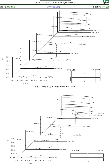
The average speed is the vector sum of velocity components, the component in component in the longitudinal direction and the normal direction. Fig.1 (on page 497) is illustrated the development of the average velocity profile for g = 0 (simulation 1) the entire length of the channel. This figure is shown the development of the flow, where after the passage of the influence of increased section there is a maximum speed of 0.12 m/s at half height of the channel. In the same section (x = 0.010m) assumes the occurrence of recirculation/stagnation of fluid caused by the unevenness of the channel.
The flow channel in the buffer zone remains constant, which is typical of a flow between two plates. As shown in the figure 4 (on page 498), the maximum average speed does not change significantly, the maximum being half the height of the channel to the section x = 0.240m. In the following section there is the division of the channel, which involves the rearrangement of the flow by the existence of solid walls, ie, the flow is forced to divide, developing differently, resulting in two new flows.
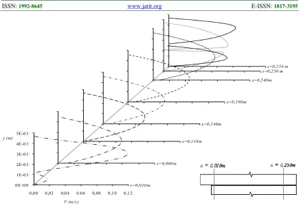
Fig. 2 (on page 497) illustrates the development of the average velocity profile along the channel for g=-gy (simulation 2). In this figure, the flow
develops in a uniform manner, with maximum average speed of almost the entire height of the channel, since the first section (x = 0.010m) to the section in which no division imposed by the flow channel geometry. In section x = 0.254m a average speed has been increased 6.5% compared to the section x = 0.250m, with a very similar development of flow in both divisions of the channel.
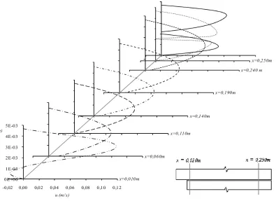
Fig.3 (on page 498) shows the development of the average velocity profile g = + gy (simulation 3) along the canal. This simulation is very similar in all the simulation 1 as can be seen by comparing Fig.1 and 3. In both simulations the influence of the value of g was evident throughout the flow and it appears on the first section (x = 0.010m) that the maximum values at mid-height of the channel differ substantially from the others. Indeed, the speed at half height of the channel is increased by about 33%. This effect, visible in simulations 1 and 3, made the profiles resemble the profiles typical of laminar flow. In the same section, as well as for simulation 1, it also raises a zone of recirculation/stagnation of fluid flow in a typical step.
The maximum speed in simulations 1 and 3 occurs in the first section (x = 0.010m) while the simulation is in section 2 x = 0.254m.
In all simulations the flow is divided, growing in solid walls, top and bottom of the channel. For simulations 1 and 3 the development of the flow is more pronounced in the upper channel while for simulation 2, although with little significant difference, the flow develops more in the lower channel.
Fig. 4 (on page 498) illustrates the development of the profile of the longitudinal component of the velocity along the channel for g = 0 (simulation 1). In this figure it is evident the development of flow in the section x = 0.010m which is after the enlargement of the channel. This step exists in the channel causes the recirculation/stagnation of fluid (Fig.5), which leads to the development of negative speeds while positive velocities in the same section. Also in this section, there is the maximum speed at half height of the channel.
The developments of flow were constant in the intermediate sections of the channel, typical of a flow between two plates. The maximum speed is half the height of the channel.
ISSN: 1992-8645 www.jatit.org E-ISSN: 1817-3195
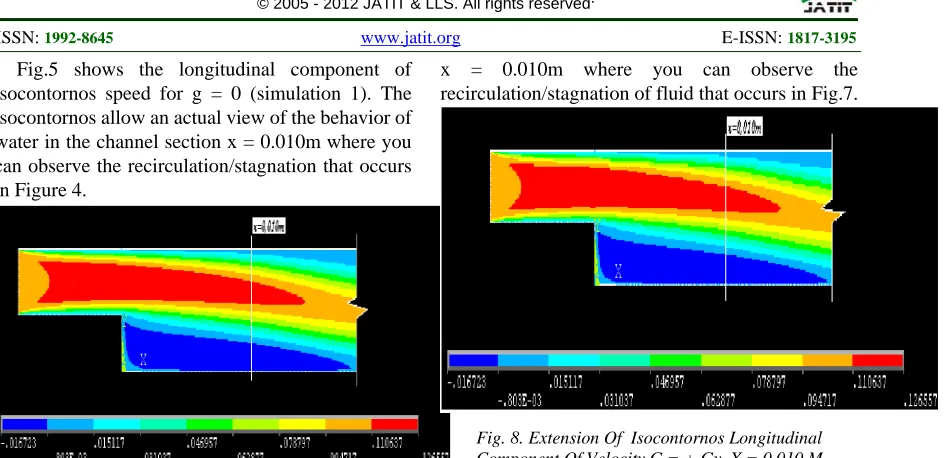
Fig.5 shows the longitudinal component of isocontornos speed for g = 0 (simulation 1). The isocontornos allow an actual view of the behavior of water in the channel section x = 0.010m where you can observe the recirculation/stagnation that occurs in Figure 4.
Figure 5. Extension Of Isocontornos Longitudinal Component Of Velocity For G = 0 In X = 0.010 M
Fig.6 (on page 499) illustrates the development of the profile of the longitudinal component of velocity along the channel to g =- gy (simulation 2). It can be seen in the figure since the first section (x = 0.010m) to the section x = 0.240mo development of the flow is constant, typical of laminar flow and is not noticeable speed changes. The maximum speed is almost the entire height of the channel.
In this simulation, as in all simulations, the presence of the recess in the channel section x = 0.250m, requires developing a shared disposal. The speed in this section and in the next section increases slightly from the previous sections, 6.5% and 14% respectively.
In section x = 0.254 m, contrary to what occurs in the section x = 0.250 m and despite being little difference, the flow is more developed than in the solid wall of the channel.
Fig.7 (on page 499) illustrates the development of the profile of the longitudinal component of velocity along the channel to gy g =- (simulation 3). This figure can be seen as very similar to Fig.4 and therefore can be viewed identical profiles, which have speed and the occurrence of recirculation/stagnation of fluid in the same section (x = 0.010m), typical of the steady flow laminar in the intermediate sections of the channel and development of two new outlets in the section x = 0.250m due to the separation channel.
Fig.8 (on page 499) shows the longitudinal component of isocontornos speed gy for g =- (simulation 3). The isocontornos allow an actual view of the behavior of water in the channel section
[image:5.612.93.565.65.294.2]x = 0.010m where you can observe the recirculation/stagnation of fluid that occurs in Fig.7.
Fig. 8. Extension Of Isocontornos Longitudinal Component Of Velocity G = + Gy, X = 0.010 M
In a simulation, as well as in simulation 3 is the maximum speed in section x = 0.010m channel, while the second simulation the peak velocity occurs in the last section analysis (x = 0.254m).
3.2 Chanel Membrane
Considering the membrane channel was made to analyze the profiles of average velocity V (m/s), the longitudinal component of velocity u (m/s) and the normal component of velocity v (m/s) at all the channel length.
Fig.9 (on page 500) illustrates the development of the average velocity profile in the channel containing membrane (simulation 4). As stated in the channel without membrane, the average velocity profile of the channel, the average speed is the vector sum of the longitudinal and normal components of velocity.
As you can see in the figure, these profiles are qualitatively similar to those observed for the situation without membrane flow in the second simulation, since the first section (x = 0.010m) to the section x = 0.190 m. In the first section, the velocity profile shows a gap caused by the change/increase in the channel strip, which assumes the occurrence of recirculation/stagnation of fluid. Along the canal the velocity profile remain almost constant which is typical of a laminar flow, the maximum occurring at mid-height of the channel.
solid wall of the channel. This is due to the fact of the membrane channel and its influence on runoff. The speed reaches its maximum value in the last section analyzed (x = 0.254m), with a value of 0.22m/s.
Fig.10 (on page 500) illustrates the development of the profile of the longitudinal component of velocity in the channel containing membrane (simulation 4). This figure is remarkable development of the flow in the section x = 0.010m which is after the enlargement of the canal, very similar to what happened in the simulations without membrane channel 1 and 3 (Fig. 4 and 7, respectively). This gap exists in the channel because recirculation/stagnation of the fluid, which leads to negative speeds development while positive velocities in the same section. Speeds also have very similar values, being in situations as described above, half the maximum height of the channel.
In section x = 0.240m view that the flow begins to take effect comportamento.Com one another in the section x = 0.250m where there is division of the channel and therefore the formation of new outlets, the longitudinal component of the velocity takes positive values solid wall near the bottom of the channel and negative values near the solid wall of the upper channel. In this section it is clear the development of preferential flow in the lower channel. The maximum speed is achieved in the last section, at the bottom of the channel.
Fig.11 (on page 501) illustrates the development of the profile of the normal component of velocity in the channel containing membrane (simulation 4). As you can see in the picture section x = 0.010m, the development of the flow has only normal component of the negative velocity with a small height of the normal component of the channel at zero speed, a result of the recirculation/stagnation of fluid observed in Figure 10 (on page 500).
The intermediate sections of the channel are not shown since they are approximately zero, and only a small development of visible flow in the section x = 0.190 m = 0.060mex. From the section x = 0.240m is clear that the existence of membrane changed significantly the behavior of the flow.
The flow in the section x = 0.250m adopts a symmetric approach, however, differently. In simulation 2 the symmetry is qualitative, the symmetry in this simulation is quantitative. In both simulations occur maximum speed in this section. In the second simulation speeds, positive and negative, arise along the solid walls of separation channel at
the top and bottom respectively, while the channel membrane velocity is maximum at the point of separation channel. The following section presents a poorly developed drainage and is only visible in the bottom of the channel, normal component of positive velocity.
ACKNOWLEDGEMENTS
This work was supported by youth key research fund of North China university of technology and KZ20110009012 .
REFERENCES:
[1] E. Mathioulakis, V. Belessiotis, and E. Delyannis, Desalination by using alternative energy: Review and state-of-the-art, Desalination, Vol.203, No.3,2007, pp.346-365.
[2] A.D. Khawaji, I.K. Kutubkanah, and J.-M. Wie, Advances in seawater desalination technologies, Desalination, Vol.221, No.1-3, 2008, pp. 47-69. [3] C. Charcosset, A review of membrane processes
and renewable energies for desalination, Desalination, Vol.245, No.1-3, 2009, pp. 214-231.
[4] R.Salcedo, E. Antipova, D. Boer,
Multi-objective optimization of solar Rankine cycles coupled with reverse osmosis desalination considering economic and life cycle environmental concerns, Desalination, Vol.286, No.1, 2012, pp. 358-371.
[5] D.F. Fletcher and D.E.Wiley , A computational fluids dynamics study of buoyancy effects in reverse osmosis, Journal of Membrane Science, Vol. 245, No. 1-2, 2004, pp.175-181.
[6] S. Wardeh and H.P.Morvan, CFD simulations of flow and concentration polarization in spacer-filled channels for application to water desalination, Chemical Engineering Research and Design, Vol.86, No.10,2008, pp. 1107-1116. [7] M.F. Gruber, C.J.Johnson and C.Y Tang,
Computational fluid dynamics simulations of flow and concentration polarization in forward osmosis membrane systems, Journal of Membrane Science, Vol.379, No.1-2, 2011, pp.488-495.
ISSN: 1992-8645 www.jatit.org E-ISSN: 1817-3195
Fig. 1. Profile Of Average Speed For G = 0
[image:7.612.106.502.387.696.2][image:8.612.90.530.394.709.2]
Fig. 3. Profile Of Average Speed For G = +Gy
ISSN: 1992-8645 www.jatit.org E-ISSN: 1817-3195
[image:9.612.97.519.76.427.2]Fig.6. Profile Of The Longitudinal Component Of Velocity G = -Gy
[image:9.612.116.511.419.706.2]Fig.9. Profile Of Average Speed For Membrane Channel
ISSN: 1992-8645 www.jatit.org E-ISSN: 1817-3195