BUS DEPATURE INTERVAL MODEL AND ALGOROTHM
UNDER THE UNCERTAIN ENVIRONMENT
1LIANG WU, 2XIAOPING GUANG
Department of Traffic and Transportation, Lanzhou Jiaotong University, Lanzhou 730070,Gansu,China
ABSTRACT
Determining the departure interval is the basic of establishing the operation plan. Based on the existing researches, and consider all kinds of uncertain factors in operation process overall, to establish a bilevel programming model which is based on the game of passengers and operation companies. And use the differential evolution bacterial foraging algorithm to solve this model. Set the passengers satisfaction as upper target, and the operational efficiency of enterprise as the lower target. At last examples show that this model can effectively optimize the departure interval, and it has certain feasibility and effectiveness.
Keywords: Bus Departure Interval, Uncertain Programming, Bilevel Programming Model, Bacterial
Foraging Algorithm
1. INTRODUCTION
With the increasingly urban traffic congestion, the public transportation gets more and more attention of people. The important component part of raising the service quality of public transport is to make the bus departure interval become more rationalization and hommization. The researches of this problem is always a hot spot in the study of the urban traffic, and scholars at home and broad do a lot of researches in public transport vehicle dispatch. The early research is mainly aimed at the enterprises or passengers as a single target and given the numerical empirical formula. Ceder[1] proposed to determine the common calculating formula of the bus departure interval and provided the optimization model and the algorithm, Banks[2] proposed to determine the departure interval model in the public transportation system and compared the interval under the changing demand of line and certain demand of line two circumstances. In recent years with the development of computer and intelligent algorithm, many scholars began to use the optimization theory to make researches [3-7], Jian Zhang started from the benefit both of the bus company and passenger and proposed a bi-level programming model of optimal route and departure interval, use intelligent algorithm to solve. Paolo [4] combined with the commonly used scheduling model of urban bus in China, established a one-dimensional nonlinear programming model and use the one-dimensional linear search method to get the approximate solution. But in the actual company operation process, due to the randomness and
uncertainty of the passengers’ travel time and space, it’s hard to achieve the rational scheduling.
2. MODEL ESTABLISHMENT
2.1 Model Assumption
Take the complete bus line which has starting and terminal station as a foundation, with the factors such as the quantity and size model of bus, to both sides (companies and passengers) maximum benefit as the goal. And in order to simplify the model, make the following assumptions[8-12]:
(1)Suppose all the optional buses model , and all of them have the same running speed on the road which is absent of the impedance.
(2)Suppose the same line operated vehicles for the same models, implement 1yuan ticket price system ,and has the same station number in uplink and downlink.
(3) Set the waiting time passengers can accept in each time interval as a constant value, and if exceed this time passengers will be unsatisfied [7]. So suppose that every time that passengers failed in waiting for buses, there will be one third of the passengers choose to other transportation, if passengers failed to get on the bus after continuously waiting for 3 buses, they will give up.
2.2 Variable And Symbolic Description
model, use the model to solve the problem in other time interval, and get the departure time.
Fixed parameters:Ν: the bus number company have(car). p :the single ticket is 1yuan. q :the station number on the route. α : seating on the bus (people). β :the maximum passengers number under the uncrowded and allowing standing situation(people). γ :the load number of the bus(people) . t :the time length of each time interval in everyday. τ :the bus departure interval(min).τ" :the maximum time of departure interval( min ). The satisfied waiting time of stations is a .
Variable: N' : the actual operating buses of company(car). hk:the bus number in uplink and down link parking lot(car). k
, i j
u :the passengers number on the bus when the jth bus pass the ith station(people). k
i,j
v :in the time interval both on the uplink and downlink the stranding passengers number when j th bus pass(people) . k
j
w :the overall number of passengers on the jth bus at both up and down direction(people). ,k
i j
r :both on the uplink and downlink ,the average satisfaction degree of waiting passengers when the j th bus pass the ith station. k,
i j
s :both on the uplink and downlink, the passengers’ average satisfaction degree to the congestion degree when the jth bus pass the ith station. ω0 :the time that passengers take when they get on or get off bus. ω ω1, 2 : separated describe the weight of the waiting passengers satisfaction degree and the weight of satisfaction degree to congestion of the passengers who are on bus. ω3 ,ω4 ,ω5:separated describe the purchase cost of unit bus on unit distance, maintenance cost and oil consumption cost.
Random variable: k, i j
λ : both on the uplink and downlink, the passengers arrival rate before the
jth bus arrival at theith station (people/min).
,
k i j
µ :both on the uplink and downlink ,the number of passengers who get off bus when the jth bus arrival at the ith(people). k
l
θ :both on the uplink and downlink ,the operation time of whole journey
l(min).
2.3 The Upper Model Establishment
The upper model take passengers’ comprehensive satisfaction degree to the bus as
goal, establish the upper objective function, and according to the antecedent hypothesis.
In the crowded condition, the number of passengers who get on bus can be expressed as:
p 1 p
, , , ,
i=1 i=2
( )
γ
k k k k
i j i j i j i j
δ = −
∑
− λ θ +∑
µ (1)The stranding passengers number at the station can be expressed as:
i-1 i
, , 1 , , , , , ,
i=1 i=2
( )
2 + 3
k k k k k k k k
i j i j i j i j i j i j i j i j
v = v − λ θ −
∑
λ θ +∑
µ −δ (2)Suppose that the average waiting time of the stranding passengers is θlk/ 2 (min ), and the passengers who are stranded at last time all get on the bus, then we can work out in one time interval on uplink or downlink, under the premise that without counting the time that passengers take on the bus ,when the jth bus pass the ith station, the average waiting time of passengers who get on bus can be expressed as:
, 1 1 , ,
,
,
( )
2
/ 2 +(s ) / 2
3
k k k k k k
i j l l i j i j l k
i j k
i j
v v
t
θ θ θ
δ − + − = − (3) Set the passengers satisfaction degree as 1 when the waiting time less than a (min ), when the waiting time greater than b (min) set it as 0. In that way when the jth bus pass the ith station the satisfaction degree of passengers who get on the bus can be expressed as:
, , , 1, a b , . a b k i j k k
i j i j t r t else ≤ = − − ; (4)
Set the satisfaction degree to crowd of passengers who have seats as 1, who have no seats set it as 0.5, In that way when the jth bus pass the
i th station the satisfaction degree to crowd of passengers who are on the bus can be expressed as :
, , , , 1, α α+0.5( α) , . k i j k k
i j i j
k i j u s u else u ≤ = − ; (5)
The comprehensive satisfaction degree of passengers can be expressed as the weighted sum of above two satisfaction degree, so the objective function of the upper model can be expressed as:
1 2
p p
2 t/τ 2 t/τ
1 , ,
1 1 i=1 1 1 i=1
max i jk i jk
k j k j
z ω r ω s
= = = =
2.4 The Lower Model Establishment
The lower model takes the operation efficiency of bus company as the objective function and establish model. Take the departure rate and capacity of bus model as decision variable. The factor of bus company’s operational invested cost include: line bus number, bus model, seats number, unit bus’s oil consumption cost and maintenance cost and so on. The main source of company operation revenue include bus fare, so lower model can be expressed as:
3 4 5
p 2 t/τ
2 ,
1 1 i=1
max k 2( )t/
i j k j
z δ ω ω ω τ
= =
=
∑∑∑
− + + (7)The first one is fare revenue, and the latter one is cost (without staff salaries).
2.5 Constraint Condition
In order to ensure there are always buses in the parking lot, so it has to satisfy that:
,
q 1 q
0 ,
1 1
· max( , k )
i j
k k
k l i j
l i
τ −θ ω λ τ µ
= =
>=
∑
+∑
⋅(N - 1) (8)
1 2 '
N≥N =N +N (9) Another constraint condition is as follows:
k ,
,
0 γ
. 3 τ τ"
0 5
i j
k i j
u
s t
v
≤ ≤ ≤ ≤
≤
≤
(10)
The first constraint condition is the constraint to the number of seating capacity in whole line, the second is the constraint to departure interval, and the third is the constraint to the number of stranded passengers, moreover, k
, τ , k i j i j
u , ,v are positive integer.
2.6 Uncertain Environment Variable
The passengers arrival rate k, i j
λ , the get off number of passengers ,
k i j
µ and the actual running time k
l
θ in whole line have uncertainty ,which is the key to determine the other parameter values, and it’s also the difficulty in public operation scheduling problem. Such as the passengers in the whole line, actually the arrival interval can translate into the combination of , k,
i j
k k
i j l
λ 、µ 、θ . Due to some parameters involve three random variable and be the nonlinear combination, therefore , in order to simplify the difficulty of the problem, simplify the above random variable as discrete random variables ,and merge the discrete point as far as possible. Through the example below can be seen, control the number of discrete point within 4, not only can effectively grasp the accuracy of the results, but
also can control the computation complexity of the model.
, q
0 ,
1
max( , k )
i j
k i j i
ω λ τ µ
=
⋅
∑
express the time thatpassengers cost on get on bus or get off the bus, in order to simplify the calculation, we suppose
, q
0 , ,
1 1
max( , k ) 1.5 ( )
i j
p
k k
i j i j
i i
ω λ τ µ λ τ
= =
⋅ =
∑
∑
.3. THE ALGORITHM
The bus scheduling problem belongs to the strong NP combinatorial optimization problem, this paper puts forward a method based on differential evolution bacteria foraging algorithm [5,8].
3.1 Coding
The bilevel programming coding is making the upper model and the lower model’s decision variables be in progress of binary hybrid coding, according to different coding segment to distinguish different decision variables, and then all of decision variable compose a binary character string. The coding content should include: the average waiting time of passengers, the degree of crowd in bus, the departure frequency, the standard busload, of which first two is decision variable of upper planning and the latter two is decision variable of lower planning .
1, 2, n
a a …,a b b1, 2,…,bn c c1, 2,…,cn d d1, 2,…,dn
Among them the a b c ii, , (i i =1, 2,, )n are
expressed as 0 or 1 binary numbers, each segment representing a decision variable.
3.2 Initialization
At first form a bacterial colony which population scale is S at a point in the space, and set the bacterial growth coefficient: the number of chemotaxis timesNC,reproduce times Nre, migration timesNedand migration probabilityPed . (1)Generate unit vector, bacteria flip. (2)According to the chemotaxis step, the bacteria swim until the adaptive value is not changed. (3)Make the differential variation. (4)Make differential cross and select.
3.3 Reproductive Growth Of Bacteria
3.4 Fitness Of Calculation
The final fitness function is F X
( )
= Cmax-f X( )
, and the f X( )
is the community scale, Cmax is arelatively large number.
The end condition is that the program should be completed after limited times of iteration, and the time is 200.
4. EXAMPLE
Now survey date to a running bus line of Lanzhou city, the route of the uplink and downlink is the same, and there are 11 station on the up and down direction. Through the survey we can get the frequency and passengers number of each interval at each station, as well as the actual operational time in each section, then put them into the model to solve the question, at last work out the optimal bus model and the departure frequency in each time interval. The table 1 is the survey date probability distribution table of number 1 station.
Tab.1 The Survey Data Probability Distribution Of Number 1 Station
Passenger arrival rateλi jk, The interval travel time θlk probability(
%)
Numerical value
probability( %)
Numerical value
70 7 85 4
30 4 15 6
For the length of article, leave out the survey date of the other station.
Suppose the seating of the preparing bus model for selecting is 20 seats, 30seats, and 40 seats, then the corresponding unit maintenance and repair cost is 100yuan, 150yuan and 200yuan. There are 4 departure interval time for selecting , respectively is 3 min ,4 min ,6 min ,and 8 min . Put all above parameter into the model to calculate, and use the differential evolution of bacteria foraging algorithm in c++ environment to calculate in program. As figure 1 shows the final result Zmax from every combination. Through the figure 1 we can see, in the corresponding interval time, using the 30 seating model and 4 minutes of departure interval can get the maximum value of the comprehensive income of both bus company benefit and society benefit.
50 60 70 80 90
3 4 6 8
[image:4.612.311.527.269.483.2]20 30 40
Fig.1 Comprehensive Benefit
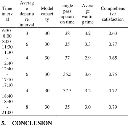
The table 2 is the determination of departure interval in each time interval and satisfaction degree value of passengers who are in buses, and set the confidence level as 0.8.
Tab.2 The Departure Intervals, The Satisfaction Of Passengers And Bus Company
Time interv al
Averag e departu
re interval
Model capaci
ty
single pass operati on time
Avera ge waitin g time
Comprehens ive satisfaction
6:30-8:00 3 30 38 3.2 0.63
8:00-11:30 6 30 35 3.3 0.77
11:30 -12:40
4 30 37 2.9 0.65
12:40 -17:10
6 30 35.5 3.6 0.75
17:10 -18:40
4 30 37.5 3.2 0.72
18:40 -21:00
8 30 35 3.0 0.79
5. CONCLUSION
The bus scheduling has greater uncertainty. This paper considered the randomness of bus scheduling. The established bilevel programming model give consideration to both company benefit and society benefit, is has a certain effectiveness and practicability. And it’s need to do more improved analysis on the intelligent scheduling to make the bus scheduling be more accurate and real time.
ACKNOWLEDGEMENTS
REFERENCES:
[1] Ceder A, “Bus frequency determination using passenger count data”, Transportation Research Part A, Vol.18, No. 5-6,1984, pp.439-453. [2] Banks J H, “Optimal headways for multi-route
transit systems”, Journal of Advanced Transportation, Vol.24, No.2,1990, pp.127-154. [3] Jian Zhang, Wenquan Li, “Bi-level programming model and algorithm for optimizing headway of public transit line”, Journal of Southeast University (English Edition),Vol.26, No.3, 2010, pp.471-474.
[4] Malachy Carey, “Optimizing Scheduled Times Allowing for Behavioral Response”, Transportation Research Part B, Vol. 32,1998, pp.329-342.
[5] Paolo Delle Site, Francesco Filippi, “Bus service optimization with fuel saving objective and various financial constraints”, Transportation Research Part A ,Vol. 35, 2001, pp.157-176. [6] A.Ceder, B.Golany, O.Tal, “Creating bus
timetables with maximal synchronization”, Transportation Research Part A, Vol. 38, 2001, pp.913-928.
[7] Christos Valouxis, Efhymios Housos, “Combined bus and driver scheduling”, Computers & Operations Research ,Vol. 29, 2002, pp.243-259.
[8] Min Wang, Yongsheng Qian, Xiaoping Guang, “Improved calculation method of shortest path with cellular automata model”, Kybernetes, Vol. 41, 2012, pp. 508-517.
[9] Ceder A, Wilson N, “Bus network design”, Transportation Research B, Vol. 20, 1986, 331- 334.
[10] Liu Y, Passino K M, “Biomimicry of social foraging bacteria for distributed optimization: Models, principles, and emergent behaviors”, Optimization Theory Application, Vol. 115, No. 3m 2002, pp. 603- 628.
[11] Das S, Biswas A, Dasgupta S, et al, “Bacterial foraging optimization algorithm: Theoretical foundations, analysis & applications”, Foundations of Computer Intel, Vol.3, 2009, pp.23- 55.