FLEXIBLE SHARING IN DHT BASED P2P NETWORKS USING METADATA OF RESOURCE

(1)

ISSN: 1992-8645 www.jatit.org E-ISSN: 1817-3195

POLE RELIABLE ASSIGNMENT

OF PARABOLIC REGION WITH ACTUATOR FAILURE

1_{BO YAO,}2_{JIAN RONG,}3_{HAO HU}

1_{College of Mathematics and System Science, Shenyang Normal University, Shenyang, 110034, P.R.}

China

2_{College of Automation Engineering, Nanjing University of Aeronautics and Astronautics, Nanjing,}

210016 P.R. China,

ABSTRACT

For a class of uncertain linear systems, this paper proposes the mixed fault model which is more general and more practical. This paper discusses the existing problems of the system reliable controller, considers the reliable pole assignment of parabolic region with actuator fault, and gives a new method to deal with the mixed fault matrix. For mixed fault model with actuator fault, it gives the sufficient condition of designing this type of controller which can make the pole of linear systems to be located in the parabolic region. It achieves the design of state feedback reliable controller by solving the LMI. The simulation proves the Design method in this paper is feasible.

Keywords: Mixed Fault Model; Pole Assignment; Actuator Fault; Parabolic Region

1. INTRODUCTION

The minimum requirement of a control system is the stability. A good controller not only transfers information fast, but also has a good response of damping events. A traditional method which can ensure system have satisfactory response, is that the poles of closed-loop system could be seated in left complex plane[1,2], and this method is called regional pole assignment. The main purpose of regional pole assignment: In the system analysis and design, the stability of the system should be considered first of all, and the instantaneous response of the linear system should be closely related with the poles’ position. It guarantees system have certain dynamic and steady-state performance, as long as the poles of the closed-loop system assign in a proper region of the complex plane. M.Chilali and P.Gahinet put forward "LMI region” firstly at 1996, afterwards, with the development of reliable control, regional pole assignment theories go deep into the reliable control gradually, and set up regional pole reliable assignment.

In fact, accurate poles assignments are not needed, it is satisfied, as long as the pole of the closed-loop system assign in a specified position of complex plane. In recent years, the pole assignment

theories of different areas are very active, for example, the pole assignment of sector region[4], circular disc region [3,6] and hyperbolic region. In fact, we can promote pole assignment of vertical or horizontal zone region toparabolic region. There is not much research about parabolic region.

Pole assignment of linear system is an important method of controller design. [3]discusses the pole assignment of circular disc with the actuator failure for linear system; [4]introduces the pole assignment of sector region for linear system. In view of the importance of regional pole assignment, it will obtain a very good development.

(2)

ISSN: 1992-8645 www.jatit.org E-ISSN: 1817-3195 complete the reliable controller design with mixed

failure model.

2. MATERIALS AND METHODS

Consider an uncertain linear system of the form

( )

(

) ( ) (

) ( )

x t



= + ∆

A

A x t

+ + ∆

B

B u t

(1) where ( )_{x t} ∈Rn

is the system state; ( )_{u t} ∈Rm_is

the actuator failure control input； _A∈Rn n× _，

Rn m

B∈ × are known constant matrices of

appropriate dimensions ； ∆A、∆B express the nondeterminacy of the system with the forms as follows :

1 2

[∆ ∆ =A B] DH E E[ ]

whereD E E, ₁, ₂ are known constant matrices of appropriate dimensions ， H is an uncertain constant matrix of appropriate dimension, which satisfies with_{H H}T ≤_I_,

Iis unit matrix.

A feedback control with the feedback gain matrixK:

( ) ( )

u t =Kx t (2)

Similarly, the actuator failure model is adopted as follows:

uf( )t =Fu t( ) (3)

where uf

( )

t ∈Rm is the actuator failure control input , Fis actuator failure model with the form as follow:

(

1 1

)

diag , , _p, _p , _n

F = n n m ₊m (4)

Let (4) be defined as follow:

i

F=N +M (5)

where N_i =diag

(

n n₁, ₂,n_p, 0,, 0

)

is called discrete failure matrix,M =diag 0,

(

, 0,m_p₊₁,m_P₊₂,

)

,m_n

 is called continuous failure matrix.

We find that the actuator failure matrix is composed of two parts, a discrete failure matrix

i

Nand continuous failure matrix M . This model is called mixed failure model.

For discrete failure matrixN_i, ifn_j =0, it means the complete failure of the j th actuator control

signal; ifn_j =1, it means normal operation of the jth actuator control signal, j=1, 2,,p.

For continuous failure matrix M , where

0≤mdi≤mi ≤mui , i=1, 2,,n with mdi≤1and 1

ui

m ≥ ,if mi =0,it means the complete failure of

the ith actuator control signal; if mi =1,it means

normal operation of the ith actuator control signal; if 0≤mdi ≤mi ≤mui , mui≥1 and mi ≠1 ,it

corresponds to the case which partial failure of the

ith control signal.

Introduce the following notations:

(

, 1

)

diag 0, , 0, , ,

u u p un

M =  m ₊  m

(

, 1

)

diag 0, , 0, , ,

d d p dn

M =  m ₊  m

(

)

0 1

2 u d

M = M +M , ₁ 1

(

)

2 u d

M = M −M

0 i 0

F =N +M

Then we have

0 1

F=F +M Σ , Σ ≤I (6)

where Σ =diag

(

σ σ₁, ₂,σn

)

, i=1, 2,n ,and

the uncertain diagonal matrixΣstands for all the diagonal matrix which can satisfy with T

I Σ Σ ≤ .

3. RESULTS AND DISCUSSIONS

Definition [10] For a region Din the complex

plane, if there exist a symmetric matrix Rn n

L∈ × and a matrix _M_∈Rn n× _{,which can make}

( )

{

T

}

: 0

D l = z∈C L+zM+zM <

thenDis called linear matrix inequality region (LMI region).

Lemma 1[11] Let D be LMI region,

and_A∈Rn n× _{, the necessary and sufficient condition}

of λ

( )

A ⊂D is that there exists a positive definite symmetric matrix _X∈Rn n× _{, which makes the}

following inequality holds:

(

)

T

(

)

T

0 L⊗ +X M⊗ AX +M ⊗ AX <

where ⊗is the symbol of Kronecker product.

(3)

ISSN: 1992-8645 www.jatit.org E-ISSN: 1817-3195 matrix_X_∈Rn n× _{, it makes the following inequality}

holds:

T T

T 2

0 2

AX XA aX AX XA

AX XA X

b

 + + − + 

 _{ <}

 ₋ ₋ 

 

 

Proof Considering the parabola lof complex plane

2

x+ = −a by

where ,a b>0are known constant.

The algebraic expression of parabolic region D l

( )

is:

( )

{

_{i :} 2_{, ,} _R

}

D l = z= +x y x+ < −a by x y∈

By z= +x iy andz = −x iy, we can get

2

z z x= + ,

2i

z z y= −

Therefore parabolic region D l

( )

can be

described as

( )

(

)

(

)

2

C : 2 0

2

b

D l =z∈ z+z + a− z−z < 

 

As

(

)

2

(

)

2 0

2

b

z+z + a− z−z < is equivalent to

(

)

(

)

2 i

0 i

2

z z a z z

b z z

 + + − − 

 _{ <}

 ₋ ₋ 

 

 

(7)

Let i 0

0 1

 

 

 and

i 0

0 1

−

 

 

 left multiply and right

multiply matrix inequality (7) respectively, then (7) is equivalent to

2

0

2

z z a z z

b z z

+ + − +

 

 _{ <}

 ₋ ₋ 

 

 

(8)

Let

2a 0

2 0 L

b

 

 

= _ ₋ _

 

, 1 1

1 0

M =  − _

  (9)

Then matrix inequality (8) can be described as:

T

0 L+zM +zM <

Because of the definition of LMI region, we know parabolic region D l

( )

is LMI region.

By Lemma 1, there exists a positive definite symmetric matrix Rn n

X∈ × , which makes the

(

)

T

(

)

T

0 L⊗ +X M⊗ AX +M ⊗ AX <

Then

( )

T T

T

2 0

0 2

0

0 ₀

aX

AX AX

AX

X _AX

b

  _ ₋ _ _ _

 ₊_ _₊_ __<

 −   

   _{ }− _

 

So we can get

T T

T 2

0 2

AX XA aX AX XA

AX XA X

b

 + + − + 

 _{ <}

 ₋ ₋ 

 

 

This paper is in order to control a state feedback

( )

u t =Kx t

for all the pole of the closed-loop system with the form as follow:

( ) (

) (

)

( )

x t =_ A+ ∆ +A B+ ∆B K x t_ (10)

( ) (

) (

)

( )

x t =_ A+ ∆ +A B+ ∆B FK x t_ (11)

are seated in parabolic LMI region.

( )

{

T

}

: 0

D l = z∈C L+zM+zM <

Lemma 2[12] X Y, are known constant matrices

with appropriate dimensions, for any constantε >0, the following inequality holds:

T T T T 1 T

XFY+Y F X ≤εXX +ε−Y Y where_{F F}T ≤_I_.

Lemma 3[13] LetF, E and Σ be real matrices of appropriate dimensions, and

(

1 2

)

diag σ σ, , σr

Σ =  with T

i i I

σ σ ≤ ,i=1, 2,,r. Then, for any real matrixΛ =diag

(

λ λ₁I, ₂I,,λ_rI

)

>0, the

T T T T T 1

F EΣ +E Σ F ≤ ΛF F +E Λ−E Considering system (1), when the actuator works normally, we have the following theorem:

Theorem 2 All the pole of the closed-loop

system (10) will be seated in parabolic regionD l

( )

,

(4)

ISSN: 1992-8645 www.jatit.org E-ISSN: 1817-3195 Rn n

X∈ × and a matrix _Y_∈Rm n× _{, which can make}

the following inequality holds:

(

)

T T T T T

1 2 1

T T T T

1 1

1

2

+ +2 0

2 0

0

0 0

aX DD DD

DD DD X

b I

I

δ δ δ

δ δ

Ψ Ψ + + Ψ − Ψ + Ξ 

 

 _{Ψ − Ψ +} ₋ _Ξ 

  <

 _Ξ ₋ 

 

 _Ξ ₋ 

 

where Ψ = AX+BY , Ξ =E X₁ +E Y₂ and the

state feedback gain matrix is_K=_YX−1_.

Proof From Theorem 1, all the pole of the

closed-loop system (10) will be seated in parabolic regionD l

( )

, if there exists a positive

definite symmetric matrixX∈Rn n× , which makes the following inequality holds:

T T T 2 2 aX X b

Ψ + Ψ + Ψ − Ψ

 _{ +}

 _{Ψ − Ψ} ₋ 

 

 

(

) (

)

T T T

1 2 , 0 + 1 2 , 0 +

D D

H E X E Y E X E Y H

D D

  ₊ ₊  

   

   

(

) (

)

T T T

1 2 1 2

0, 0, 0

0 0

D D

H E X E Y E X E Y H

− −

  ₊ ₊ ₊   _<

   

   

(12)

whereY =KX ,Ψ =AX +BY .

From lemma 2, there existsδ δ >₁, ₂ 0, inequality (12) can be included in the following inequality

T T T 2 + 2 aX X b

Ψ + Ψ + Ψ − Ψ

 

 _{Ψ − Ψ} ₋ 

 

 

(

) (

T

)

1

1 1 1 2 , 0 1 2 , 0

T

D D

E X E Y E X E Y

D D

δ    ₊δ− ₊ ₊ ₊

     

(

) (

T

)

1

2 2 0, 1 2 0, 1 2 0

0 0

T

D D

E X E Y E X E Y

δ − −  ₊δ− ₊ ₊ _<

  

  

(13)

Using the Schur complement, matrix inequality (13) is equivalent to the conclusion of Theorem2. And it is obvious that the state feedback gain matrix isK =YX−1by the process of proof above.

Considering the system (1) with actuator failure, we have the following theorem:

Theorem 3 All the pole of the closed-loop

system (11) will be seated in parabolic region

( )

D l , if there exists a positive definite symmetric

matrix_X_∈Rn n× _{, a matrix}_Y_∈_Rm n× _{and positive}

definite symmetric matricesU V, ∈Rm m× , which make the following inequality holds:

11 12 13 14

T

12 22 23 24

T T

13 23 33

T T

14 24 44

0 0

0

Φ Φ Φ Φ

 

_Φ _Φ _Φ _Φ 

 _{ <}

Φ Φ Φ 

 

Φ Φ Φ

 

where

T T T T

1 2 1

11 T T T

1 1

( ) 2

2 +

DD aX DD

DD DD X

b

ε ε ε

ε ε

Π + Π + + + Π − Π + + 

 

Φ = _ _{Π − Π} ₋ _

 

T T T T T

1 0 2

12 T T T T T

1 0 2

0 0

X E Y F E

 + 

Φ =  

+  ， T 1 13 1 = 0

BM U Y BM U

 

Φ  

  1 14 T 0 = 0 BM V Y  

Φ  ₋ 

  ， 1 22 2 0 0 I I ε ε −  

Φ =  ₋ 

  ， 2 1 23 0 = 0 0

E M U

 

Φ  

  24 2 1 0 0 = 0 E M V

 

Φ _ _

−

  , 33

0 0 U U −  

Φ =  ₋ 

  ， 44 0 0 V V −  

Φ =  ₋ 

 

0

AX BF Y

Π = +

and the state feedback gain matrix isK=YX−1.

Proof From Theorem 1, all the pole of the

closed-loop system (11) will be seated in parabolic region D l

( )

, if there exists a positive definite

symmetric matrix X∈Rn n× .And letY =KX , we can get

T T T T T T T T

T T T T

2

AX BFY XA Y F B aX XA Y F B AX BFY

AX BFY XA Y F B X

b  + + + + + − −   _{ +}  ₊ ₋ ₋ ₋     

(

) (

)

T T T

1 2 , 0 + 1 2 , 0 +

D D

H E X E FY E X E FY H

D D

   

+ +

   

   

(

) (

)

T T T

1 2 1 2

0, 0, 0

0 0

D D

H E X E FY E X E FY H

− −

   

+ + + <

   

   

(14)

(5)

T T T T T T T T

T T T T

2

+ 2

AX BFY XA Y F B aX XA Y F B AX BFY

AX BFY XA Y F B X

b  + + + + + − −     ₊ ₋ ₋ ₋     

(

) (

T

)

1

1 1 1 2 , 0 1 2 , 0

T

D D

E X E FY E X E FY

D D

ε    ₊ε− ₊ ₊ ₊

     

(

) (

T

)

1

2 2 0, 1 2 0, 1 2 0

0 0

T

D D

E X E FY E X E FY

ε − −  ₊ε− ₊ ₊ _<

  

  

(15)

Using the Schur complement and (6), matrix inequality (15) is equivalent to can be describe as

(

)

T T T T T T T T T 1 2 1 1 0 2

T T T T T T T T

1 1 1 0 2

1 2 0 1

1 2 0 2

2 0

2

+ 0

0 0

DD aX DD X E Y F E

DD X DD X E Y F E

b

E X E F Y I

ε ε ε

ε ε

ε

Π +Π + + + Π −Π + + 

 

 _{Π −Π} ₋ ₊ ₊ 

 +  ₊ ₋     ₊ ₋   

(

) (

)

T 1 1 T

1 T 1

2 1 2 1

, 0, 0, 0 + , 0, 0, 0

0 0

BM BM

Y Y

E M E M

   

   

 _Σ _Σ   ₊

           

(

) (

)

T 1 1 T T

2 1 2 1

0 0

0, , 0, 0 0, , 0, 0 0

0 0

BM BM

Y Y

E M E M

   

   

 _Σ ₋ ₊ ₋ _Σ   _<

   

₋  ₋ 

   

(16)

whereΠ =AX+BF Y₀ .

From lemma 3, there exist positive definite symmetric matrices , Rm m

U V∈ × which make

inequality (16) be included in the following inequality:

(

)

T T T T T T T T T 1 2 1 1 0 2

T T T T T T T T

1 1 1 0 2

1 2 0 1

1 2 0 2

2 0

2

+ 0

0 0

DD aX DD X E Y F E

DD X DD X E Y F E

b

E X E F Y I

ε ε ε

ε ε

ε

Π + Π + + + Π −Π + + 

 

 _{Π −Π} ₋ ₊ ₊ 

   ₊ ₋     ₊ ₋   

(

)

(

)

T 1 1 T 1

2 1 2 1

0 0

+ 0, , 0, 0 0, , 0, 0

0 0

BM BM

V Y V Y

E M E M

−            _{ + −} ₋         − −    

(

)

(

)

T 1 1 T

1 1 1

2 1 2 1

, 0, 0, 0 , 0, 0, 0 0

0 0

BM BM

U Y U Y

E M E M

−

   

   

+_ _{ } _ + <

   

   

(17)

Using the Schur complement, we conclude matrix inequality (17) is equivalent to the conclusion of Theorem 3. And it is obvious that the

state feedback gain matrix is _K₌_YX−1 _{by the}

process of proof above.

4. NUMERICAL EXAMPLE

In this section, we present a numerical example for actuator failure to illustrate the proposed design method.

Consider the linear system (1) with the following parameters

0.9 1.7 2.2 0.5 3.7 1.6 2.5 1.6 4.2 A −     =_ − − _  ₋ ₋    ,

0.2 1 0.3

3.5 0.8 1.6 5 1.8 1.5 B − −     = −_ − _  ₋ ₋ ₋   

0.1 0 0.2

0 0.15 0.1

0 0 0.4

D     =       , ₁

0.5 0 0

0 0.5 0

0 0 0.5

E     =       2

0.4 0.1 0.2

0.2 0.5 0.2

0.6 0.6 1

E     =      

,f_u₃ =2.4, f_d₃ =0.8

0.2

a= ,b=0.5 (18) The poles of the system which is determined by (19) set for

{

-6.6510,0.2322,-2.3812

}

, so nominal

system is unstable.

(I) When the actuator of system (18) works normally, according to theorem 2, the reliable control gain matrix is:

0.4560 0.0246 0.4777

0.4910 0.5061 0.5133 0.6881 0.6435 1.3519 K     =   ₋ ₋ ₋   

By the reliable controller which designed in theorem 2, the pole of closed-loop system (10) will be seated in the region, as in Figure 1:

Fig 1

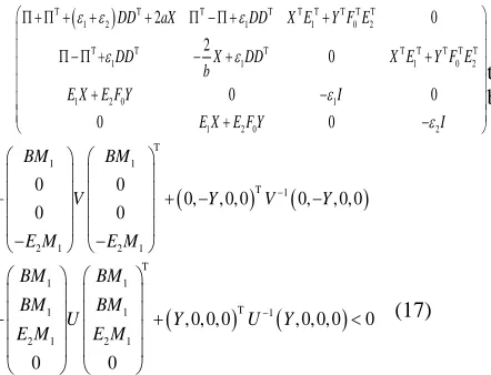
(II) When The Actuator Of System (18) Has Failure, Let Discrete Fault Matrix

(

)

1 diag 1, 0, 0

[image:5.612.94.315.515.684.2]

(6)

ISSN: 1992-8645 www.jatit.org E-ISSN: 1817-3195 By the controller which designed in theorem 2,

[image:6.612.89.525.124.524.2]

the pole of closed-loop system (11) will not be seated in the region, as in Figure 2, 3, 4:

[image:6.612.331.520.138.520.2]

Fig 2. For Closed-Loop System (11), Distribution Of The Pole WithN=N1

Fig 3. For Closed-Loop System (11), Distribution Of The Pole WithN=N₂

Fig 4. For Closed-Loop System (11), Distribution Of The Pole WithN=N3

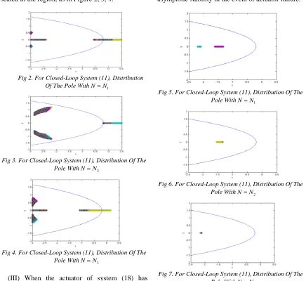
(III) When the actuator of system (18) has failure, according to theorem 3, the reliable control gain matrix is:

0.5293 0.3573 0.5982

1.3324 0.2401 0.7605

0.1673 0.0393 0.1003

K

 

 

=  

 ₋ ₋ 

 

The pole of closed-loop system (11) will be seated in the region, as in Figure 5, 6, 7:

Simulation results show that, when uncertain linear system (1) does not have failure, it is stable by the controller designed in theorem 2. However when system (1) has actuator failure, it is unstable

as the controller designed in theorem 2. But the reliable controller with mixed failure model which designed by theorem 3 will have a good and stable performance, not only when all control components

are operational, but also in case of some admissible control component outages. It ensures the system’s asymptotic stability in the event of actuator failure.

5. CONCLUSION

[image:6.612.107.297.139.484.2]

(7)

REFERENCES

[1] B.C.Kuo, 1982. Automatic Control Systems. Englewood Cliffs, NJ: Prentice-Hall.

[2] Hu Hao and Yao Bo,2011.Robust

pole assignment of circular disc for a class of continuous interval system. Computing Technology and Automation, 30(2):17-20. [3] Hu Hao,Yao Bo and Huang Shan,2011.Robust

Circular Pole Assignment for A Class of Discrete Interval Systems. Proc. of CCDC2011, pp:575-580.

[4] I.R.Petersen, 1987, A stabilization algorithm for a class of uncertain linear System.Syst., 08:351- 357.

[5] J.Ackermann, 1993. Robust Control: Systems with Uncertain Physical Parameters. London, Springer-Verlag.

[6] M.Chiali and P.Gahinet, 1996. H∞ design with pole placement constraints: an LMI approach.IEEE Transactions on Automatic Control, 41(3): 358-367.

[7] R.J.Veillette,J.V.Medamic and W.R.Perkins, 1992. Design of reliable control systems.IEEE Transactions on Automatic Control, 37(3):770-784.

[8] Wang Jianhua and Yao Bo, 2010.Design of reliable controller with mixed fault model in linear systems.IEEE, Proc.of CCDC2010, pp:1709- 1712.

[9] Yao Bo and Sun Xin, 2004.Reliable Control Pole Assignment of Quadrant Region.Proc.of the 5th World Congress on Intelligent Control, pp: 39 - 42.

[10] Yao Bo, Wang Fuzhong and Zhang Siyang, 2008 .Pole Reliable Assignment of Circular Disc With Actuator Fault. CCDC2008, pp: 463 -466.

[11] Yang G H,Wang J L and Soh Y

C,2001.Reliable H_∞control for linear systems . Automatica, 37(3):717-725

[12] Yu Li, 2002.Robust Control-Linear Matrix Inequality Approach.Beijing, pp: 96-100.

[13] Y.S.Lee,Y.S.Moon,W.H.Kwon and

P.G.Park,2004. Delay-dependent robust H_∞ control for uncertain systems with a state-delay. Automatica, pp.65-72.