R E S E A R C H
Open Access
Random sampling and approximation of
signals with bounded derivatives
Jianbin Yang
1*and Xinzhu Tao
1*Correspondence:
1Department of Mathematics,
College of Science, Hohai University, Nanjing, China
Abstract
Approximation of analog signals from noisy samples is a fundamental, but
nevertheless difficult problem. This paper addresses the problem of approximating functions inHγ,Ωfrom randomly chosen samples, where
Hγ,Ω=
f|fis continuous on
Ω
, andDfL∞(Ω)≤γ
fL∞(Ω).
We are concerned with the probability that functions inHγ,Ωcan be approximated
from the noisy samples stably and how they can be approximated.
By calculating the upper bound of the covering number of a subset ofHγ,Ωand
using the uniform law of large numbers, we conclude that functions inHγ,Ωcan be
recovered stably with overwhelming probability provided that the sampling noise satisfies some mild conditions and the sampling size is sufficiently large. Furthermore, an
∞-regularized least squares model is proposed to approximate functions from noisy samples. The alternating direction method of multipliers (ADMM) algorithm is then applied to solve the model. In the end, numerical experiments are presented and discussed to illustrate the efficiency of our method.
MSC: 42C40; 60E15; 94A20; 62D05
Keywords: Sampling inequalities; Signals with bounded derivatives; Covering number; Regularized least squares
1 Introduction
In modern digital data processing of signals, such as sound, image or video processing, one always uses a discretized version of the original analog functions [1]. Then how the ana-log function can be recovered from its samples and whether the reconstruction is stable are fundamental problems in sampling theory [2]. For example, the Shannon–Whittaker sampling theorem says for eachf ∈L2(R) andsupp(fˆ)⊆[–12,12], it can be completely
re-covered from the sample points{f(j) :j∈Z}by the formulaf(x) =j∈Zf(j)sinππ(x(–xj–)j), where the convergence is uniform onRand also inL2(R).
To characterize the conditions under which it is possible to recover particular classes of functions from the sampling points stably, we introduce the following sampling inequali-ties:
mpfpLp(Rd)≤
xj∈X
f(xj) p
≤MpfpLp(Rd) ∀f ∈V, (1.1)
wherempandMpare positive constants independent off and 1≤p<∞. The setX={xj:
j∈J}is said to be a stable set of sampling for function classV⊆Lp(Rd) if the inequalities
(1.1) hold (see e.g. [2,3]). The sampling inequalities (1.1) imply that a small perturbation off causes only a small change of sampled values{f(xj)}, and vice versa. This means that
the sampling is a stable process and the reconstruction of functions inV fromXis con-tinuous. For the Shannon–Whittaker theorem, since the functions{sinππ(·(–·j–)j)}j∈Zform an
orthonormal basis for the space of bandlimited functions with highest cycle frequency12, we havef2L2(R)=j∈Z|f(j)|2andm
2=M2= 1.
In the past years, there has been a considerable body of research on developing recon-struction algorithms and characterizing the conditions of stable set of sampling for various function classes. For instance, Aldroubi and Gröchenig [2] investigated the nonuniform sampling and reconstruction in shift-invariant spaces. Xian and Li [4,5] studied the sam-pling set conditions and applications of weighted finitely generated shift-invariant spaces. Sun and Zhou [6], and Sun [7] characterized the local sampling in spline subspaces and shift-invariant spaces, respectively.
This paper addresses the problem of sampling and approximation of functions with bounded derivatives. We define the following class of functions onΩ⊂Rd:
Hγ,Ω:=
f |f is continuous onΩ, andDfL∞(Ω)≤γfL∞(Ω)
, (1.2)
where|Df|=|Dx1f|+|Dx2f|+· · ·+|Dxdf|, andDxi= ∂
∂xiis the weak derivative of order 1.
The continuity of f at the boundary ofΩ means thatf can be continuously extended toΩ. The parameterγ characterizes the degree of oscillation of functions inHγ,Ω. For
simplicity, throughout this paper, we always assume thatΩ= (0, 1)d. Sampling inHγ ,Ω is
an appropriate model for many applications, in particular in signal and image processing [1]. Moreover, by Bernstein’s inequality [8], iff ∈L2(R) andsupp(fˆ)⊆[–4γπ,
γ
4π], thenf ∈ Hγ,R. In other words, the space of bandlimited functions is a special case ofHγ,Ω.
Random sampling approaches were used in a variety of fields, such as statistical learn-ing theory [9], compressed senslearn-ing [10], image processlearn-ing [11], and many others [12]. Re-cently, Bass and Gröchenig in [13] studied the stability problem of random sampling in the space of bandlimited functions. Yang et al. [14,15] and Führ et al. [16] discussed the stability conditions and applications of random sampling in shift-invariant spaces.
The purpose of this paper is to investigate random sampling of functions in Hγ,Ω.
Let{(xj,yj)}nj=1 be the sampling off ∈Hγ,Ω, where{xj}is uniformly drawn fromΩ, and
yj=f(xj) +jwithj being a random noise. We consider the probability that{(xj,yj)}nj=1
is a stable set of sampling forHγ,Ω, and howf can be approximated from these samples.
By estimating the upper bound of the capacity ofHγ,Ω and applying the uniform law of
large numbers of the sampling values, we conclude that with overwhelming probability, the sampling inequalities (1.1) hold uniformly for all functions inHγ,Ωwhen the sampling
noise satisfies some mild conditions. Furthermore, an∞-regularized least squares model is proposed, and the corresponding numerical algorithm is discussed.
The rest of this paper is structured as follows. Section2introduces some mathematical notation and the covering number ofHγ,Ω. Section3characterizes the stability properties
of random sampling inHγ,Ω. Section4.1presents an optimization model and the
corre-sponding numerical algorithm to approximatef ∈Hγ,Ωfrom its noisy samples. Section4.2
2 Preliminaries
We first introduce some notation. LetNdenote the set of positive integers. As usual, for
x∈R, let xdenote the largest integer smaller than or equal tox, andxdenote the smallest integer greater than or equal tox. For x= (x1, . . . ,xd), y= (y1, . . . ,yd)∈Rd, let
|x–y|:=max1≤i≤d{|xi–yi|}.
For two setsAandB, the Cartesian productA×Bis the set of all ordered pairs defined byA×B={(a,b)|a∈Aandb∈B}. Similarly, it can be generalized to anm-ary Cartesian product overmsets.
LetMbe a Lebesgue measurable set. For 1≤p<∞, we denote byLp(M) the Banach
space of all functions such that
fLp(M):=
M
f(x)pdx
1/p
<∞ for 1≤p<∞,
andfL∞(M)is the essential supremum off onM.
We can similarly definep=p(Zd) the Banach space of all sequencesa= (ak)k∈Zd such
thatap<∞, where
ap:=
k∈Zd |ak|p
1/p
for 1≤p<∞,
anda∞is the supremum ofaonZd.
The first main result of this paper is to estimate the probability such that the sampling inequalities (1.1) hold uniformly for all functions inHγ,Ω. Such similar problems are
clas-sical in statistical learning theory [9]. The most powerful tool used there is the capacity of the involved function set and the uniform law of large numbers [17–19]. Our analysis is following this strategy.
Since the covering number is a very convenient and powerful tool for metric space, we choose it to characterize the capacity of function sets. LetSbe a metric space. For any
η> 0, the covering numberN(S,η) is the minimal number of balls with radiusηthat can coverS. WhenSis compact,N(S,η) is finite for any givenη> 0.
It is not hard to verify that any f ∈Hγ,Ω satisfies the inequalities (1.1) if and only if f/fL∞(Rd)does. So we consider the subset
Hγ∗,Ω:=f ∈Hγ,Ω, andfL∞(Ω)= 1
. (2.1)
The following proposition gives an upper bound for the covering number ofHγ∗,Ω, and the proof follows the line of argument in [9, Proposition 5.4] whered= 1.
Proposition 2.1 Let Hγ∗,Ω be defined by(2.1).For anyη> 0,the covering number of Hγ∗,Ω with respect to · L∞
NHγ∗,Ω,η
≤exp
ln2 +2
η+
4γ η
d
ln3 .
that the point set
X:=xi= (xi1,xi2, . . . ,xid)|xi=iδ,i∈I
d
is a regular grid inΩwith equal distanceδ, which is also aδ-net ofΩ.
Forf∈Hγ∗,Ω, we haveDfL∞≤γfL∞≤γ. Moreover, by the continuity off, for any
x,y∈Ω, we have –1≤f(x)≤1 and|f(x) –f(y)| ≤γ|x–y|. It follows that
(νi– 1) η
2 ≤f(xi)≤νi
η
2, ∀xi∈X,
for someνi∈J :={–2η+ 1, –2η+ 2, . . . ,η2}. For each
ν= (ν(1,1,...,1),ν(2,1,...,1), . . . ,νi, . . . ,ν( 1
δ,
1
δ,...,
1
δ))∈J
|Id|,
define
Hν:=
f∈Hγ∗,Ω(νi– 1) η
2≤f(xi)≤νi
η
2,∀i∈I
d
.
Then we obtain
Hγ∗,Ω⊆
ν∈J|Id| Hν.
Besides, for everyf,g∈Hν, there exist˜i∈Idandx˜
i∈Xsuch that
max
x∈Ω
f(x) –g(x)= max
|x–x˜i|≤δ
f(x) –g(x)
≤ max
|x–x˜i|≤δ
f(x) –f(x˜i)+g(x) –g(x˜i)+f(x˜i) –g(x˜i)
≤2γ δ+η 2=η.
Hence, we conclude that the diameter ofHν⊆Hγ∗,Ωis at mostη, and
Hν:ν∈J|Id|
is anη-covering ofHγ∗,Ω.
In the following, we count the number of sets{Hν},ν∈J|Id|. Letf∈Hν. For every fixed
i= (i1,i2, . . . ,i, . . . ,id)∈Idandxi∈X, we have
(νi– 1) η
2 ≤f(xi)≤νi
η
2.
Similarly, forxi∈X withi= (i1,i2, . . . ,i+ 1, . . . ,id)∈Id, aδ-neighboring point ofxi, we
have
(νi– 1)η
2 ≤f(xi)≤νi
η
It follows that
(νi–νi– 1) η
2≤f(xi) –f(xi)≤(νi–νi+ 1)
η
2. (2.2)
Sincef∈Hν⊆Hγ∗,Ω and|xi–xi|=δ, we have f(xi) –f(xi)≤γ δ=
η
4. (2.3)
By (2.2) and (2.3), we obtain|νi–νi|
η
2–
η
2≤
η
4. Hence,
νi∈ {νi,νi+ 1,νi– 1}.
In addition, sinceν(1,1,...,1)has at most 2η2possible values, the number of nonempty sets
{Hν},ν∈J|Id|is at most
2
2
η
3|Id|≤2
2
η+ 1 3 1
δd
≤exp
ln
2
2
η+ 1
+
1
δ d
ln3
≤exp
ln
2
2
η+ 1
+
4γ η
d
ln3 .
Moreover, sinceln(1 +t)≤tfort≥0, we have
exp
ln
2
2
η+ 1
+
4γ η
d
ln3 ≤exp
ln2 +2
η+
4γ η
d
ln3 .
This completes the proof of Proposition2.1.
3 Stability of random sampling
LetX={xj:j∈N}be a sequence of independent and identically distributed (i.i.d.)
ran-dom variables, each of which is uniformly drawn fromΩ, andyj=f(xj) +jwithjbeing
a random noise. In this section, we investigate the probability that anyf ∈Hγ,Ω can be
recovered from its samples{(xj,yj)}nj=1stably. We will prove that if the random noise
satis-fies some mild conditions, then, with overwhelming probability, the sampling inequalities (1.1) hold uniformly for all functions inHγ,Ω with (noisy) sampling values.
For every fixedf ∈Hγ,Ω, we define the random variable
Xj(f) :=f(xj)p–
Ω
f(x)pdx, (3.1)
where{xj}is uniformly drawn fromΩ. Then one can check that the sequence{Xj(f) :j∈N}
is independent and the expectationE(Xj(f)) = 0. Besides, for the variance ofXj(f), we have
VarXj(f)
=EXj(f)2
–EXj(f) 2
=Ef(xj) 2p
–
Ω
f(x)pdx
≤Ef(xj) 2p
=
Ω
f(x)2pdx
≤ f2p L∞(Ω).
The following Bernstein inequality plays an important role in probability theory, which gives bounds on the probability that the sum of independent random variables deviates from the expectation.
Lemma 3.1([20]) Letξ1,ξ2, . . . ,ξnbe independent random variables.Assume thatE(ξj) =
0,Var(ξj)≤σ2and|ξj| ≤K almost surely for all j.Then,for anyλ≥0,
Prob 1 n n j=1 ξj ≥λ
≤2exp
– nλ
2
2σ2+2 3Kλ
.
Lemma 3.2 Let{xj:j= 1, 2, . . . ,n}be a sequence of i.i.d.random variables that are
uni-formly drawn fromΩ= (0, 1)d.Let Hγ∗,Ω be defined by(2.1),and Xj(f)be given by(3.1).
Then,for anyλ≥0and n∈N,
Prob
sup
f∈Hγ∗,Ω 1 n n j=1
Xj(f) ≥λ
≤2N
Hγ∗,Ω,
λ
2p exp
– 3nλ
2
24 + 4λ .
Proof Let{f}=1,...,L, where L=N(Hγ∗,Ω, λ
2p), be a sequence in Hγ∗,Ω such thatHγ∗,Ω can
be covered by theL∞ balls centered atfwith radius 2λp. For each fixedf∈Hγ∗,Ω, since fL∞(Ω)= 1, we haveVar(Xj(f))≤1 and|Xj(f)| ≤1. By Lemma3.1, we obtain
Prob 1 n n j=1
Xj(f) ≥λ
≤2exp
– nλ
2
2 +23λ . (3.2)
For any givenf ∈Hγ∗,Ω, there exists some∈ {1, 2, . . . ,L}such thatf–fL∞≤2λp. Thus,
by the mean value theorem,
1 n n j=1
Xj(f) –
1
n
n
j=1
Xj(f) = 1 n n j=1 f(xj)
p
–f(xj) p
≤pmaxfL∞(Ω),fL∞(Ω) p–1
f –fL∞(Ω)
≤pf –fL∞(Ω)
≤λ
Combining this with (3.2), we conclude that, for each fixed, 1≤≤L,
Prob
sup
{f:f–fL∞≤2λp}
1 n n j=1
Xj(f) ≥λ ≤Prob 1 n n j=1
Xj(f) ≥λ–
λ
2
≤2exp
– 3nλ
2
24 + 4λ .
Besides, since
Hγ∗,Ω⊆
L
=1
f :f –fL∞≤ λ 2p , we obtain Prob sup
f∈Hγ∗,Ω 1 n n j=1
Xj(f) ≥λ ≤ L =1 Prob sup
{f:f–fL∞≤2λp}
1 n n j=1
Xj(f) ≥λ
.
Therefore, noting thatL=N(Hγ∗,Ω, λ
2p), we conclude that
Prob
sup
f∈Hγ∗,Ω 1 n n j=1
Xj(f) ≥λ
≤2N
Hγ∗,Ω,
λ
2p exp
– 3nλ
2
24 + 4λ .
Theorem 3.3 Let Hγ,Ω be defined by(1.2).Assume that{xj:j= 1, 2, . . . ,n}is a sequence
of i.i.d.random variables that are uniformly drawn fromΩ.Then,for any0 <λ< 1
(p+1)dγd, the following sampling inequalities:
n1 – (p+ 1)dγdλ
Ω
f(x)pdx≤
n
j=1 f(xj)
p
≤n1 + (p+ 1)dγdλ
Ω
f(x)pdx (3.3)
hold uniformly for all functions in Hγ,Ωwith probability at least
1 – 2exp
ln2 +4p
λ +
8pγ λ
d
ln3 – 3nλ
2
24 + 4λ .
Proof Obviously that everyf ∈Hγ,Ω satisfies (3.3) if and only iff/fL∞ does. Thus, we
assume thatfL∞= 1 andf ∈Hγ∗,Ω.
LetXj(f) be defined by (3.1), and one can check that the event
E=
sup
f∈Hγ∗,Ω 1 n n j=1
Xj(f) ≥λ
is the complement of
˜ E= n Ω
f(x)pdx–λn≤
n
j=1 f(xj)
p
≤n
Ω
f(x)pdx+λn,∀f∈Hγ∗,Ω
For an arbitraryf ∈Hγ∗,Ω, there exists anx∈Ωsuch that|f(x)|=fL∞= 1. Without
loss of generality, we assume thatf(x) = 1. Then, forx∈Ω∗, whereΩ∗:={x∈Ω,|x–x| ≤
1
γ}, we have
fx–f(x) =f(x) –fx≤γx–x≤1.
It follows that
f(x)≥1 –γx–x≥0 forx∈Ω∗
and
Ω
f(x)pdx≥
Ω∗
1 –γx–xpdx≥ 1
(p+ 1)dγd.
Therefore, the event
¯ E=
n1 – (p+ 1)dγdλ
Ω
f(x)pdx≤
n
j=1 f(xj)
p
≤n1 + (p+ 1)dγdλ
Ω
f(x)pdx,
∀f ∈Hγ∗,Ω
contains the eventE˜.
Thus, by Lemma3.2and Proposition2.1, the inequalities (3.3) hold uniformly for all functions inHγ,Ω with probability
Prob(E¯)≥Prob(E˜) = 1 –Prob(E)
≥1 – 2exp
ln2 +4p
λ +
8pγ λ
d
ln3 – 3nλ
2
24 + 4λ .
Corollary 3.4 Under the same conditions of Theorem3.3,let yj=f(xj) +j,j= 1, 2, . . . ,n
be the sampling of f.Suppose that the random noise{j}are independent with E(|j|p) =σp
and||j|p–σp| ≤MfpLpfor allj.In addition,we assume that σp
fpLp ≤ρ1.Then,for
any0 <λ<21–p2(p1–+1)p–dργd+1,the inequalities
n21–p–ρ–21–p(p+ 1)dγd+ 1λ
Ω
f(x)pdx
≤
n
j=1
f(xj) +jp
≤2p–1n1 +ρ+(p+ 1)dγd+ 1λ
Ω
f(x)pdx (3.4)
hold uniformly for all functions in Hγ,Ωwith probability at least
1 – 2exp
–nλ
2
2M2
1 – 2exp
ln2 +4p
λ +
8pγ λ
d
ln3 – 3nλ
2
24 + 4λ
Proof One can check that everyf ∈Hγ,Ω satisfies the inequalities of (3.4) if and only if f/fLpdoes. Thus, we assume thatfLp= 1. By Hoeffding’s inequality [21], we have
Prob
1
n
n
j=1
|j|p–σp ≥λ
≤2exp
–nλ
2
2M2 .
So, with probability 1 – 2exp(–2nMλ22),
1
n
n
j=1
|j|p≤σp+λfpLp.
For 1≤p<∞, sincetp is a convex function ofton [0, +∞), by Jensen’s inequality, we
have
f(xj) +jp≤f(xj)+|j| p
≤2p–1f(xj)p+|j|p
and
f(xj) +j p
≥f(xj)–|j| p
≥21–pf(xj) p
–|j|p.
Hence, with the same probability, we have
n
j=1
f(xj) +j p
≤2p–1
n
j=1 f(xj)
p
+ 2p–1nσp+λfpLp
and
n
j=1
f(xj) +j p
≥21–p
n
j=1 f(xj)
p
–nσp+λfpLp.
Combining this with Theorem3.3, we conclude that
n21–p–ρ–21–p(p+ 1)dγd+ 1λ
Ω
f(x)p
dx
≤
n
j=1
f(xj) +jp
≤2p–1n1 +ρ+(p+ 1)dγd+ 1λ
Ω
f(x)pdx
holds with probability at least
1 – 2exp
–nλ
2
2M2
1 – 2exp
ln2 +4p
λ +
8pγ λ
d
ln3 – 3nλ
2
24 + 4λ
.
We remark thatρin Corollary3.4is connected with the signal-to-noise ratio (SNR) of
4 Approximation algorithm and numerical examples
4.1 Approximation model and algorithm
In this subsection, we consider how to approximate f ∈Hγ,Ω from its noisy samples {(xj,yj)}nj=1, whereyj=f(xj) +jandj is a random noise. The main idea is that we seek
an approximantf∗by solving the following optimization problem:
min
g∈V n
i=1
g(xi) –yi 2
+Γ(g), (4.1)
where the first term tries to fitf∗(xi) toyi, and the second term is a regularization term.
For the function spaceV in (4.1), there are several choices, such as the Sobolev space, reproducing kernel Hilbert space, polynomial space or a principal shift-invariant space
Sh(φ,Ω), which is defined by
Sh(φ,Ω) =
α∈I
u(α)φ ·
h–α : u(α)∈R
,
with
I=
α∈Zd:suppφ
·
h–α ∩Ω=∅
.
Here, functionφis called the generator ofSh(φ,Ω), andh> 0 is a scaling parameter that
controls the refinement of the space. The compact support ofφis preferred since it gener-ates sparse matrices. In addition,Sh(φ,Ω) provides good approximation to smooth func-tions ifφsatisfies certain conditions (see e.g. [22–24]).
The regularization term in (4.1) is chosen such that the derivative off∗ is controlled and the sampling noise can be reduced. For g =α∈Iu(α)φ(h· –α), we take Γ(g) =
diag(λ)Wu∞, whereWis the discrete wavelet frame transform, anddiag(λ) is a diag-onal matrix based on the vectorλwhich scales different wavelet channels. The advantage of using wavelet frames here is that the model has fast algorithms, and wavelet frames can be regarded as certain discretizations to the general differential operator [25]. Moreover, with properly chosen parametersdiag(λ), we haveDgL∞(Ω)∼ diag(λ)Wu∞[26].
In summary, we determine the approximating function by minimizing
n
j=1
α∈I
u(α)φ
xj
h –α –yj
2
+diag(λ)Wu
∞, (4.2)
where u are the coefficients to solve. Finally, let
f∗=
α∈I
u∗(α)φ ·
h–α
with u∗being the minimizer of (4.2).
Next, we show how to numerically solve (4.2), which can be written in the following matrix-vector form:
min
u∈RmAu– y
2
where y = [y1,y2, . . . ,yn]T, Ajk=φ(xj/h–αk),X={x1, . . . ,xn}andI={α1, . . . ,αm}. This is
equivalent to
min
u,d Au– f 2
2+diag(λ)d∞ subject to d =Wu. (4.4)
Then the alternating direction method of multipliers (ADMM) method [12,25] can be applied to solve (4.4) as follows:
⎧ ⎪ ⎪ ⎪ ⎨ ⎪ ⎪ ⎪ ⎩
ui+1=arg min
uAu– f22+
μ
2Wu– di+ bi 2
2, (4.5)
di+1=arg min
ddiag(λ)d∞+μ2d–Wui+1– bi22, (4.6)
bi+1= bi+Wui+1– di+1, (4.7)
with initial guesses u0, d0, b0and a parameterμ.
The quadratic problem (4.5) has the first order optimality condition
2ATA+μIu= 2ATf+μWTdi– bi. (4.8)
This is a sparse and positive definite linear system, and we use the conjugate gradient (CG) method to solve the problem. The solution to (4.6) is equivalent to the proximal operator of · ∞, i.e.,
proxλ μ·∞
Wui+1+ bi= arg min d
d∞+ μ 2λd–
Wui+1+ bi2
2.
By the property of the Moreau decomposition [12],
proxλ μ·∞
Wui+1+ bi=Wui+1+ bi– projB1(0,λ μ)
Wui+1+ bi,
where projB1(0,λ
μ)is the projection to the1-norm ball given by
projB1(0,λ
μ)(t) = arg min
v1≤λμ
v– t22. (4.9)
The exact solution of (4.9) can be computed at mostO(N) time [27], whereNis the di-mension of the space.
Note that the numerical computation ofWT(di– bi) in (4.8) is done by fast wavelet
algo-rithm, similar to (4.6) and (4.7); see [25,28] for detailed discussions. Finally, the proposed algorithm is summarized in Algorithm1.
4.2 Numerical examples and discussions
In this subsection, we show the efficiency of the proposed approach (4.2) by approximating two functions inHγ,Ωfrom some noisy samples.
In the first example, we test to approximate the well-known Franke function [29], which is defined as follows:
franke(x1,x2) =
3 4e
–((9x1–2)2+(9x2–2)2)/4+3
4e
–((9x1+1)2)/49–(9x2+1)/10
+1 2e
–((9x1–7)2+(9x2–3)2)/4–1
5e
Algorithm 1∞-regularized least squares algorithm
Initialize:Set initial guesses d0, u0and b0. Choose an appropriate set of parametersμ
andλ. Given a toleranceε> 0. Seti= 0. whiledi–Wui
2≥ do
ui+1= (2ATA+μI)–1(2ATf+μWT(di– bi))
di+1=Wui+1+ bi– proj
B1(0,λμ)(Wui+1+ bi)
bi+1= bi+Wui+1– di+1
[image:12.595.112.480.79.378.2] [image:12.595.136.334.474.557.2]i=i+ 1 end while
Figure 1Approximation of 1000 samples from the Franke function
We randomly sample {xj}1000j=1 from Ω = (0, 1)2, and take the sampling values yj =
franke(xj)+j, wherejis a random variable drawn from the normal distributionN(0, 0.01).
Set the scaling parameterh= 1/180, and the tensor product of the cubic spline
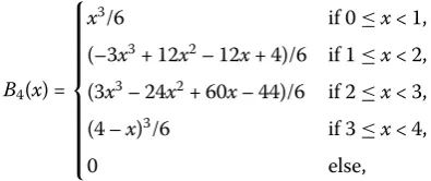
B4(x) = ⎧ ⎪ ⎪ ⎪ ⎪ ⎪ ⎪ ⎪ ⎪ ⎨ ⎪ ⎪ ⎪ ⎪ ⎪ ⎪ ⎪ ⎪ ⎩
x3/6 if 0≤x< 1,
(–3x3+ 12x2– 12x+ 4)/6 if 1≤x< 2,
(3x3– 24x2+ 60x– 44)/6 if 2≤x< 3,
(4 –x)3/6 if 3≤x< 4,
0 else,
as generatorφ, with its associated wavelet tight frame masksh1= [1/16, –1/4, 3/8, –1/4,
1/16],h2= [–1/8, 1/4, 0, –1/4, 1/8],h3= [
√
6/16, 0, –√6/8, 0,√6/16] andh4= [–1/8, –1/4,
0, 1/4, 1/8].
Figure 1(a) illustrates the approximation result obtained by Algorithm 1, whereas Fig.1(b) shows the original Franke function. It can be seen that the proposed model (4.2) is able to approximate function well.
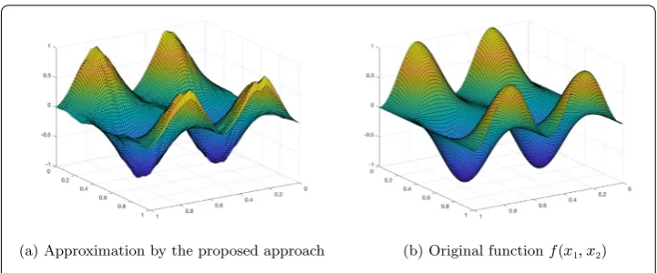
In the second example, we test to approximate
f(x1,x2) =sin(2πx1)2cos(2πx2). (4.10)
Using a similar method to the first example, we randomly sample{xj}1000j=1 fromΩ= (0, 1)2
Figure 2Approximation of 1000 samples fromf(x1,x2) (4.10)
same generatorφand parameterh. In Fig.2(a) the approximation is depicted, whereas in Fig.2(b) the original functionf(x1,x2) is depicted.
5 Conclusion and future work
In this paper, we investigated random sampling of functions with bounded derivatives. We considered the probability that functions inHγ,Ω can be recovered from noisy samples
stably and how they can be approximated.
For the stability problem, we first estimated the capacity ofHγ,Ω. By using the uniform
law of large numbers, we concluded that functions inHγ,Ω can be recovered stably with
overwhelming probability when the sampling noise satisfies some mild conditions. Then we proposed an∞-regularized least squares model in order to control the fluctuation of functions and suppress noise. The ADMM algorithm was applied to solve the optimization model. Finally, experiments on some function approximation tasks indicate the efficiency of the proposed approach.
In future work, it is of interest to present an error analysis for different kinds of denoising schemes when they are applied to reconstructing functions from random sampling.
Acknowledgements
The authors thank Prof. Qiyu Sun at University of Central Florida and Prof. Jun Xian at Sun Yat-Sen University for valuable discussions on the sampling of signals with bounded derivatives.
Funding
This work was partially supported by the National Natural Science Foundation (Grant No. 11771120) and the Fundamental Research Funds for the Central Universities 2018B19614, China.
Availability of data and materials Not applicable.
Competing interests
The authors declare that they have no competing interests.
Authors’ contributions
All authors contributed equally to the manuscript and approved the final manuscript.
Publisher’s Note
Springer Nature remains neutral with regard to jurisdictional claims in published maps and institutional affiliations.
References
1. Lapidoth, A.: A Foundation in Digital Communication, 2nd edn. Cambridge University Press, Cambridge (2017) 2. Aldroubi, A., Gröchenig, K.: Nonuniform sampling and reconstruction in shift-invariant spaces. SIAM Rev.43(4),
585–620 (2001)
3. Xian, J.: Average sampling and reconstruction in a reproducing kernel subspace of homogeneous type space. Math. Nachr.87(8–9), 1042–1056 (2014)
4. Xian, J., Li, S.: Sampling set conditions in weighted finitely generated shift-invariant spaces and their applications. Appl. Comput. Harmon. Anal.23(2), 171–180 (2007)
5. Xian, J., Li, S.: Improved sampling and reconstruction in spline subspaces. Acta Math. Appl. Sin. Engl. Ser.32(2), 447–460 (2016)
6. Sun, W., Zhou, X.: Characterization of local sampling sequences for spline subspaces. Adv. Comput. Math.30(2), 153–175 (2009)
7. Sun, Q.: Local reconstruction for sampling in shift-invariant spaces. Adv. Comput. Math.32(3), 335–352 (2010) 8. Pinsky, M.A.: Introduction to Fourier Analysis and Wavelets, vol. 102. Am. Math. Soc., Providence (2008)
9. Cucker, F., Zhou, D.-X.: Learning Theory: An Approximation Theory Viewpoint. Cambridge University Press, Cambridge (2007)
10. Candès, E.J.: Compressive sampling. In: Proceedings of the International Congress of Mathematicians, vol. 3, pp. 1433–1452 (2006)
11. Piazzo, L.: Image estimation in the presence of irregular sampling, noise, and pointing jitter. IEEE Trans. Image Process.
28(2), 713–722 (2019)
12. Boyd, S., Parikh, N., Chu, E., Peleato, B., Eckstein, J.: Distributed optimization and statistical learning via the alternating direction method of multipliers. Found. Trends Mach. Learn.3(1), 1–122 (2011)
13. Bass, R.F., Gröchenig, K.: Random sampling of bandlimited functions. Isr. J. Math.177(1), 1–28 (2010) 14. Yang, J., Wei, W.: Random sampling in shift-invariant spaces. J. Math. Anal. Appl.398(1), 26–34 (2013) 15. Yang, J.: Random sampling and reconstruction in multiply generated shift-invariant spaces. Anal. Appl.17(2),
323–347 (2019)
16. Führ, H., Xian, J.: Relevant sampling in finitely generated shift-invariant spaces. J. Approx. Theory240, 1–15 (2019) 17. Wu, Q., Ying, Y., Zhou, D.-X.: Learning rates of least-square regularized regression. Found. Comput. Math.6(2), 171–192
(2006)
18. Cai, J.F., Shen, Z., Ye, G.B.: Approximation of frame based missing data recovery. Appl. Comput. Harmon. Anal.31(2), 185–204 (2011)
19. Lin, S., Guo, X., Zhou, D.-X.: Distributed learning with regularized least squares. J. Mach. Learn. Res.18(1), 3202–3232 (2017)
20. Bennett, G.: Probability inequalities for the sum of independent random variable. J. Am. Stat. Assoc.57(297), 33–45 (1962)
21. Hoeffding, W.: Probability inequalities for sums of bounded random variables. J. Am. Stat. Assoc.58(301), 13–30 (1963)
22. Jia, R.Q.: Approximation with scaled shift-invariant spaces by means of quasi-projection operators. J. Approx. Theory
131(1), 30–46 (2004)
23. Dong, B., Shen, Z.: Pseudo-splines, wavelets and framelets. Appl. Comput. Harmon. Anal.22(1), 78–104 (2007) 24. Johnson, M.J., Shen, Z., Xu, Y.H.: Scattered data reconstruction by regularization in B-spline and associated wavelet
spaces. J. Approx. Theory159(2), 197–223 (2009)
25. Cai, J.F., Osher, S., Shen, Z.: Split Bregman methods and frame based image restoration. Multiscale Model. Simul.8(2), 337–369 (2009)
26. Yang, J., Stahl, D., Shen, Z.: An analysis of wavelet frame based scattered data reconstruction. Appl. Comput. Harmon. Anal.42(3), 480–507 (2017)
27. Duchi, J., Shalev-Shwartz, S., Singer, Y., Chandra, T.: Efficient projections onto the1-ball for learning in high dimensions. In: Proceedings of the 25th International Conference on Machine Learning, pp. 272–279. ACM, New York (2008)
28. Dong, B., Shen, Z.: MRA Based Wavelet Frames and Applications. IAS Lecture Notes Series. Summer Program on The Mathematics of Image Processing, Park City Mathematics Institute (2010)