Improving Power System Voltage Stability by Using Demand Response
to Maximize the Distance to the Closest Saddle-Node Bifurcation
Mengqi Yao, Ian A. Hiskens, and Johanna L. Mathieu
Abstract— Temporal load shifting via demand response can be used to improve power system frequency stability. Recent work has shown that spatio-temporal load shifting can also be used to improve power system static voltage stability. However, the best static voltage stability metric is an open question. In this paper, we propose a method to improve power system static voltage stability by maximizing the distance to the closest saddle-node bifurcation of the power flow. Specifically, we formulate a nonlinear nonconvex optimization problem in which we choose loading patterns that maximize this distance while also constraining the total system loading to remain constant so that the actions do not affect frequency stability. We derive the KKT conditions and solve the resulting nonlinear system of equations using the Newton-Raphson method and check if the solution is a local minimum. Using a 4-bus system and the IEEE 9-bus system as our test cases, we explore the performance of the algorithm and the accuracy of the obtained solutions. We compare the solution to those obtained using other voltage stability metrics including the smallest singular value of the power flow Jacobian and the loading margin, finding that all approaches produce different solutions. Using Kundur’s two area system, we also explore some algorithm convergence issues.
I. NOTATION
Sets
SPV Set of all PV buses
SPQ Set of all PQ buses
SDR Set of buses with demand responsive loads
Variables & Parameters θi Voltage angle at busi
Vi Voltage magnitude at bus i
Pi Real power injection at busi
Qi Reactive power injection at busi
d Distance to the closest Saddle-Node Bifurcation
x System state vector
λ System parameter vector (power injections)
Λ Feasible set of λ
ndr Number of buses with demand responsive loads
ne Number of engineering limits
m Length of system state and parameter vectors
w Left eigenvector corresponding to zero eigenvalue
αi Ratio between real and reactive demand at busi
β Weighting matrix
µ, γ Lagrange multipliers
ζ Constant
This research was funded by NSF Grant #ECCS-1549670. The authors are with the Department of Electrical Engineering & Computer Science, Uni-versity of Michigan, Ann Arbor, MI 48109 USA.{mqyao, hiskens, jlmath}@umich.edu
Functions
F(·):Rm×Rm→Rm Standard power flow
g1(·): Rndr→
R2ndr Demand response limits
g2(·): Rm→Rne Engineering limits
h(·): R2ndr→
Rndr+1 Demand response assumptions We use the superscript ‘c’ to denote states/parameters at the closest Saddle-Node Bifurcation (SNB), the superscript ‘?’ to denote states/parameters at the solution, and the super-script ‘0’ to denote states/parameters at the initial operating point. For notational simplicity, we assume that each bus has at most one generator or one load. The notationX 0
means thatX is a positive definite matrix.
II. INTRODUCTION
Demand response can be used to improve power system economics and reliability [1]. There has been a significant amount of recent research into the development of strategies that enable demand response resources to provide frequency regulation via temporal load shifting, e.g., [2], [3]. However, demand response can also be used to improve other types of power system stability, for example, static voltage stability via load shedding [4] and spatio-temporal load shifting [5], [6]. Spatio-temporal load shifting refers to increas-ing/decreasing the load at various points in the network while forcing the total loading to remain constant and then paying back the load changes in future time intervals. In this way, frequency stability is unaffected because the total loading is unchanged in every time period. Additionally, each load receives the same amount of energy over the entire horizon as it would have received without demand response.
The best static voltage stability metric is an open question. Our previous research investigated use of the loading margin [7] and the smallest singular value (SSV) of the power flow Jacobian [8] within the spatio-temporal load shifting problem [5], [6]. However, the loading margin specifies the direction of the changes to power injections precipitating an instability and the SSV gives only indirect information about the distance to instability [9].
series compensation) to improve this distance. The benefit of this approach is that the resulting optimization problem can be solved by formulating the Karush-Kuhn-Tucker (KKT) conditions, solving the nonlinear system of equations using the Newton-Raphson method, and checking if the solution is a local minimum by using the iterative method proposed in [13]. By reinitializing the nonlinear system solver and repeating this process many times we may find the global minimum, though we have no guarantee. We note that, in practice, limit-induced bifurcations (LIB) may occur before SNBs. We do not consider LIBs here; in future work we will explore algorithmic approaches to maximize the distance to the closest SNB or LIB.
Our contributions are as follows. 1) We formulate the optimization problem and derive its KKT conditions. 2) We conduct case studies using a 4-bus system and the IEEE 9-bus system and explore the performance of the algorithm and the accuracy of the solution. In particular, we find that our algorithm is able to maximize the distance to the globally closest SNB for the 4-bus system but does not find the globally closest SNB for the 9-bus system, instead maximizing the distance to a locally closest SNB. However, the globally closest SNB of the 9-bus system is unrealistic. 3) We compare our solution to those obtained by formulations that use other stability metrics. We find that all approaches produce different results and we discuss the implications of this finding. 4) Using Kundur’s two area system, we explore algorithm convergence issues.
The remainder of this paper is organized as follows. Section III describes the problem. Section IV reviews the optimization formulation used for finding the closest SNB. Section V formulates our problem and presents our solution approach. Section VI shows the results of our case studies and Section VII concludes the paper.
III. PROBLEMDESCRIPTION
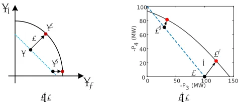
A conceptual illustration of the problem is shown in Fig. 1. The power flow solvability boundary (black curve) is defined by a set of SNBs, whereλdenotes power injections. Suppose the initial operating point with injections equal toλ0 is not sufficiently far from its closest SNB. The system operator would like to increase this distance, which is a measure of static voltage stability. It could do so through generator redisptach, load shedding, and/or spatial load shifting. Here, we investigate the impact of spatial load shifting.
While generators take time to respond to dispatch com-mands, demand responsive loads can respond quickly if coordinated via low-latency communications systems. Load shedding reduces quality of service to consumers and re-quires an equivalent decrease in generation to maintain system frequency. In contrast, spatial load shifting decreases and increases loads at various points in the network while maintaining the total loading so as not to affect system frequency. Aggregations of loads such as residential and commercial air conditioning systems can both decrease and increase their power consumption for short periods of time. So long as the energy is “paid back” within a short period of time, quality of service can be maintained. While it would likely be uneconomical to purpose-build demand response
λ
1λ
2λ0
λ*
λc
d*
(a)
0 50 100 150 -P3 (MW) 0
20 40 60 80 100
-P4
(MW)
λ* λc
d* λ0
[image:2.612.319.556.56.158.2](b)
Fig. 1. Illustration of the problem. The black curve is the power flow solvability boundary and the dashed line shows the feasible solutions.λ0
is the initial operating point;λ? is the optimal operating point with the
maximum shortest distance to the boundary andλc is the corresponding
closest SNB. (a) Conceptual illustration. (b) 4-bus system example. capability for this application, it could be one of many services that demand responsive loads could provide in future power networks.
In Fig. 1a, the blue dashed line is the feasible range of the injections, including the requirement that the total loading is constant. Our goal is to determine injectionsλ?
corresponding to the optimal operating point along the blue dashed line that maximize the distanced?to the closest SNB
λc. Figure 1b shows an example using a simple four bus
system that will be discussed in detail in Section VI-A. The optimization problem is:
max
λ?⊂Λ?
min
λc⊂Λc||
λc−λ?||2
, (1)
whereΛdefines the feasible set ofλ.
In our formulation, we assume that the generator real power outputs do not change with the exception of that of the slack bus, which changes its output to compensate for the change in system losses that occurs when the load is spatially shifted. (Alternatively, we could have assumed that the total load plus losses remain constant, i.e., that the loads manage the change in system losses and none of the generator real power outputs change.) Additionally, we assume that PV bus voltages are fixed. Therefore, we choose only the real and reactive power consumption of each demand responsive load, which is modeled as constant power with constant power factor. In practice, the system operator could simultaneously redispatch generators and demand responsive loads to im-prove the stability margin, though the generators may be ramp limited. However, here we focus on characterizing the response of demand responsive loads alone.
IV. CLOSESTSADDLE-NODEBIFURCATIONS
We first review the approach for computing the closest SNB to a given operating point. The standard power flow equations [14] can be expressed as:
F(x, λ) =f(x)−λ= 0, (2)
where x ∈ Rm is the system state vector, λ ∈
Rm is the system parameter vector and F : Rm×Rm → Rm. In this paper, we assume x = [θi∈SPV; θi∈SPQ; Vi∈SPQ] and
singular:
∂fT
∂x w= 0, (3)
where w ∈ Rm is a left eigenvector corresponding to the zero eigenvalue of the power flow Jacobian matrix. To obtain a unique solution of w, we normalized the left eigenvector such thatwTw−1 = 0.
As discussed in [10], for a given operating point(x0, λ0), if the distance to bifurcation is defined as Euclidean distance
d = ||λc −λ0||2, then the closest SNB can be found by solving the following optimization problem:
min
xc,λc,w 1 2||λ
c−λ0||2
2 (4a)
subject to F(xc, λc) = 0 (4b)
∂fT
∂x
(x=xc)w= 0 (4c)
wTw−1 = 0. (4d)
To solve (4), we derive the KKT conditions. The Lagrange function is:
L=1 2||λ
c
−λ0||22+µ
T
1F(x
c, λc) +µT
2
∂fT
∂x
(x=xc)w
+µ3(wTw−1), (5)
whereµ1∈Rm,µ2∈Rm,µ3∈Rare Lagrange multipliers. Therefore, the KKT conditions are:
∂L ∂xc =µ
T
1
∂f ∂x
(x=xc)+µ
T
2
∂ ∂x
∂fT
∂x w
(x=xc)= 0 (6a) ∂L
∂λc = (λ c
−λ0)T +µT1∂F
∂λ = 0 (6b)
∂L ∂w =µ
T
2
∂fT ∂x
(x=xc)+ 2µ3w
T = 0 (6c)
(4b)−(4d) (6d)
From (6b) we know thatµT
1∂F/∂λ6= 0. Also,∂F/∂λ=
−I. Therefore, the Lagrange multiplierµ1must be nonzero. If we post-multiply (6c) by w, the first term becomes zero and since w is not zero, µ3 must be zero. Then µ2 is either zero or a right eigenvector corresponding to the zero eigenvalue of the power flow Jacobian (making the first term of (6c) zero). Assumeµ2 is a right eigenvector. Post-multiplying (6a) by µ2 results in the first term becoming zero, and therefore the second term, which has quadratic form, must also equal zero. This is only possible ifµ2 lies in the null space of the (symmetric) matrix of that second term. Accordingly, the second term of (6a) must equal zero. Alternatively, if µ2 = 0 then that second term in (6a) is zero. In either case, the first term of (6a) must equal zero, so µ1 must be a left eigenvector corresponding to the zero eigenvalue of the power flow Jacobian. Since both µ1 and
ware left eigenvectors corresponding to the zero eigenvalue of the power flow Jacobian, we can set µ1 = ζ1w, where
ζ16= 0 is a scalar.
Hence, a locally closest SNB must satisfy the following equations:
F(xc, λc) = 0 (7a)
∂fT
∂x
(x=xc)w= 0 (7b)
wTw−1 = 0 (7c)
(λc−λ0)−ζ1w= 0. (7d)
Reference [10] proposed a similar set of equations, the only difference being that instead of (7d) they use the more general equation (λc−λ0)−(∂FT/∂λ)w = 0 since they
allowλto be any system parameter whereas we defineλas power injections. Equation (7) is a set of 3m+ 1nonlinear equations with 3m + 1 unknowns. Direct methods, for instance, the Newton-Raphson method, or iterative methods such as the one given in [15] can be used to compute the numerical solutions to (7). Note that the KKT conditions are just necessary conditions giving us minima, maxima, and saddle points. Solutions obtained with Newton-Raphson need to be checked to ensure they are minima. In contrast, the iterative method in [15] guarantees that the solution is a local minimum, i.e., a locally closest SNB. The distance to the locally closest SNB isd=||λc−λ0||
2=||ζ1w||2=|ζ1|. We can attempt to find the globally closest SNB by computing all of the locally closest SNBs using different initializations and determining the minimum d. This may be computationally intractable for large systems and we have no guarantee that we will obtain the globally closest SNB.
V. OPTIMIZATIONFORMULATION
In our problem, we need to determine both the parameters
λ? corresponding to the optimal operating point and the
parametersλc corresponding to the closest SNB. Since the real power injections at PV buses and the real and reactive power injections at PQ buses without demand responsive loads are unchanged, we divide λ? into two parts. The
controlled power injections λ?
1 = [Pi∈SDR; Qi∈SDR] are limited by the flexibility of the demand responsive loads:
g1(λ?1) =
Pi−Pi, ∀i∈ SDR
−Pi+Pi,∀i∈ SDR
≤0, (8)
where g1 : R2ndr →
R2ndr and P
i, Pi are the
lower and upper limits of the range of allowed changes to the real power consumption of the demand respon-sive loads. The uncontrolled power injections are λ?2 =
[Pi∈SPV; Pi∈SPQ\SDR; Qi∈SPQ\SDR] =λ 0 2. Our goal is to determine λ?
1 that maximizes the distance to its closest SNB. Therefore, the decision variables of the optimization problem are the system state vectors xc, x?, system parameter vectorsλc, λ?
1 and the left eigenvectorw. The optimization problem is:
min
xc,λc,x?,λ?
1,w
−1 2(λ
c−λ?)Tβ(λc−λ?) (9a)
subject to F(xc, λc) = 0 (9b)
F(x?, λ?) = 0 (9c)
∂fT
∂x
(x=xc)w= 0 (9d)
wTw−1 = 0 (9e)
g1(λ?1)≤0 (9g)
g2(x?)≤0. (9h)
The objective (9a) maximizes a weighted distance instead of the Euclidean distance (β 0). Constraints (9b) and (9c) are the standard power flow equations for the SNB and the optimal operating point, respectively. Constraint (9d) implies that (xc, λc) is an SNB. The left eigenvector w
is normalized in (9e). Equation (9f) ensures our demand response assumptions are enforced at λ?
1, specifically, 1) the total loading is constant and 2) the load is modeled as constant power with constant power factor:
h(λ?1) =
P
P? i∈SDR−
PP0
i∈SDR
αiPi?−Q?i,∀i∈ SDR
= 0, (10)
where h: R2ndr →
Rndr+1. The inequality constraint (9g) is defined in (8). The inequality constraint (9h) specifies the engineering limits at (x?, λ?). They include limits on the
voltage magnitudes at PQ buses, the reactive power injections at PV buses and the slack bus, and the line flows (g2:Rm→ Rne). The Lagrange function of (9) is:
L=−1 2(λ
c−λ?)Tβ(λc−λ?) +µT
1F(x
c, λc)
+µT4F(x?, λ?) +µT2∂f
T
∂x
(x=xc)w+µ3(w
Tw−1)
+µT5h(λ?1) +γT1g1(λ?1) +γ
T
2g2(x?), (11) whereµ1, µ2, µ4∈Rm, µ3∈R,µ5∈Rndr+1,γ1∈R2ndr andγ2∈Rneare Lagrange multipliers. The KKT conditions are:
∂L ∂xc =µ
T
1
∂f ∂x
(x=xc)+µ
T
2
∂ ∂x
∂fT
∂x w
(x=xc)= 0
(12a)
∂L ∂λc =−(λ
c−λ?)TβT +µT
1
∂F
∂λ = 0 (12b)
∂L ∂x? =µ
T
4
∂f ∂x
(x=x?)+γ
T
2
∂g2
∂x
(x=x?)= 0 (12c) ∂L
∂λ?1 = (λ
c
1−λ
?
1)
TβT
1 +µ
T
4
∂F ∂λ1
+µT5 ∂h ∂λ?1 +γ
T
1
∂g1
∂λ?1 = 0
(12d)
∂L ∂w =µ
T
2
∂fT
∂x1
(x=xc)+ 2µ3w
T = 0 (12e)
equality constraints (9b)−(9f) (12f)
γ1,jg1,j(λ?1) = 0,∀j= 1, ...,2ndr (12g)
γ2,kg2,k(x?) = 0,∀k= 1, ..., ne (12h)
γ1≥0, γ2≥0 (12i)
inequality constraints (9g)−(9h) (12j)
As before,µ1equals a constant timesw, i.e., µ1=ζ2w, the second term of (12a) is equal to zero, andµ3= 0. Therefore, an optimal solution should satisfy the following equations:
µT4
∂f ∂x
(x=x?)+γ
T
2
∂g2
∂x
(x=x?)= 0 (13a) −β(λc−λ?)−ζ2w= 0 (13b)
β1(λc1−λ?1) +
∂FT
∂λ1
µ4+
∂hT ∂λ?
1
µ5+
∂gT1
∂λ?
1
γ1= 0 (13c)
equality constraints (12f)−(12h) (13d)
inequality constraints (12i)−(12j), (13e)
whereβ1is the partition ofβcorresponding toλ1. There are
5m+ 5ndr+ne+ 2equations and unknowns in (13a)-(13d). The solution algorithm is as follows. First, we initialize the Newton-Raphson solver to find the solution to (13a)-(13d). We check to see if the solution also satisfies (13e). If so, we check whetherλcis a locally closest SNB toλ?by using the iterative method of [15]. If so, then we check whetherλcis a
globally closest SNB toλ?by testing different initializations
within the iterative method to determine if there is a closer SNB to λ? than λc. If we find that λc is the globally
closest SNB thenλ? is the desired solution. Otherwise, we reinitialize the Newton-Raphson solver in the direction of the globally closest SNB to find a new λ? and repeat the process.
In our cases studies, we compare the performance of our method to that of a brute force method. Specifically, for all possible loading patterns within a discrete mesh in which the total loading is constant, we compute the distance to the closest SNB via the method of [15]. The optimal loading pattern is the pattern associated with the maximum distance.
VI. CASESTUDY
All computation is done in MATLAB and with the help of MATPOWER[16] on an Intel(R) i7-4720HQ CPU with 16 GB of RAM. The base MVA for all cases is 100 MVA and we set β = I. The number of the equality constraints greatly influences the computation time of our method, therefore, we neglect (9h) in our case studies. In each case, our initial operating points satisfy (9h) and we also find that the optimal solutions we obtain also satisfy (9h).
A. Simple 4-bus system results
We first apply our method to the simple 4-bus system as shown in Fig. 2a. Bus 1 is the slack bus at a voltage of 1 pu, bus 2 is a PV bus outputting 10 MW at a voltage of 1 pu, and buses 3 and 4 are PQ buses with demand responsive loads of 30 MW and 70 MW, respectively. The reactance of the lines arex13=j0.5, x23=x34=j0.25p.u.
Whenλonly includes the real power injections at the PQ buses (i.e.,λ= [P3; P4]), the solution is as shown in Fig. 1b. Specifically, the black curve is the power flow solvability boundary; the dashed blue line represents the total loading constraint, i.e., P3 +P4 = −100 MW; and the optimal loading pattern is λ? = [−100,0] MW, which maximizes
the shortest distance to the boundary.
If we instead defineλ= [P2−4; Q3−4], the initial distance to the closest SNB is d = 0.0879. The optimal solution determined by our method isP?
3 =−63.74MW and P4?=
−36.26MW, and d?= 0.1264, which is consistent with the
optimal loading pattern obtained via the brute force method, as shown in Fig. 2b.
B. IEEE 9-bus system results
TABLE I
IEEE 9-BUSSYSTEM:INITIAL AND OPTIMAL POWER INJECTIONS(P.U.)
P2 P3 P4 P5 P6 P7 P8 P9 Q4 Q5 Q6 Q7 Q8 Q9
λ0 1.6300 0.8500 0.0000 -0.9000 0.0000 -1.0000 0.0000 -1.2500 0.0000 -0.3000 0.0000 -0.3500 0.0000 -0.5000 λc 1.0629 0.2508 -0.1248 -1.5821 -0.6003 -1.3436 -0.5726 -1.7980 -0.2961 -0.7620 -0.0638 -0.3343 -0.0741 -0.9325
λ? 1.6300 0.8500 0.0000 -1.0842 0.0000 -0.7386 0.0000 -1.3272 0.0000 -0.3614 0.0000 -0.2585 0.0000 -0.5309
~
~ 1
2 3 4
(a)
0
-P3 (MW) 0
0.02 0.04 0.06 0.08 0.1 0.12 0.14
d
20 40 60 80 100
[image:5.612.71.285.274.414.2](b)
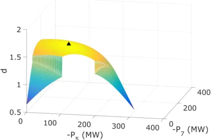
Fig. 2. (a) Single line diagram for the 4-bus system. (b) The distance to the closest SNB as a function ofP3.
Fig. 3. The distance to the closest SNB as a function ofP5andP7. buses (buses 4-9). We model the entire load at buses 5, 7 and 9 (315 MW) as demand responsive. Hence, the system parameter vector is λ = [P2−9;Q4−9] and the controlled power injections are λ?
1 = [P5?;P7?;P9?;Q?5;Q?7;Q?9]. We assume the system is initially operating at the operating point given within MATPOWER (see Table I,λ0).
The optimal solution obtained by our method is given in Table I. The corresponding maximum distance is d?
β =
1.6263, the optimal loading pattern isP5 =−108.42MW,
P7 =−73.86 MW, and P9 =−132.72 MW. To verify the results, we compare the solution of our method to that of the brute force method. We use 5000 different directions as initializations of the iterative method of [15] to find locally closest SNB to λ? and then determine the globally closest
SNB. Figure 3 shows the distance to the closest SNB as a function ofP5 andP7 (whereP9=−315−P5−P7 since the total loading must be constant). The triangle represents the maximum distance obtained by the brute force method:
P5 = −108 MW, P7 = −74 MW, P9 = −133 MW and d = 1.6263, which is consistent with the solution of our method. There exist discontinuities on the surface in Fig. 3 because the feasibility boundary is very likely a folded hypersurface, so the distance is not continuous.
We have verified that λc is a locally closest SNB to
λ? but we cannot guarantee that this SNB is the globally
TABLE II
VOLTAGE AND REACTIVE POWER(P.U.)AT THESNBS
V4 V5 V6 V7 V8 V9 Q1 Q2 Q3
SNB 1 0.5618 0.1593 0.5812 0.0795 0.4969 0.3571 7.8432 8.2343 7.1842 SNB 2 0.7780 0.6907 0.9071 0.8841 0.9009 0.6946 4.9147 1.6245 1.5874
closest SNB since the brute force method only explores 5000 random directions. Recently, [17] proposed a new enumer-ation search strategy to identify multiple local minima to a related optimization problem. Applying this strategy to (4), we obtain a closerλc to ourλ?with a distanced= 0.1718. This solution satisfies the KKT conditions (7) and may be the globally closest SNB to λ?. The voltage magnitudes
at the PQ buses and the reactive power injections at the buses with generators corresponding to this SNB (SNB 1) and the SNB that our method finds (SNB 2) are given in Table II. For both, the voltage magnitudes are low and the generator reactive power injections are high; however, SNB 1 is particularly unrealistic. Our method moves the system away from the relatively realistic locally closest SNB (SNB 2) but unfortunately there is a closer SNB (SNB 1), which it does not find. This example points to one of the drawbacks of our approach: we cannot guarantee that we will find the globally closest SNB so we might push the system away from a locally closest SNB and end up closer to the globally closest SNB.
TABLE III
OPTIMAL LOADING PATTERNS FOR DIFFERENT STABILITY METRICS
−P5 −P7 −P9 SSV LM d
(MW) (MW) (MW) – (MW) (p.u.) max SSV 75 167 73 0.8995 516 1.5819 max LM 97 135 83 0.8984 566 1.6033 maxd 108 74 133 0.8898 408 1.6263
0 500 1000 1500 2000 2500 3000
-P7 (MW) 500
1000 1500 2000
-P9
(MW)
Power flow solvability bounday
*,1
*,opt c,1
0 *,2
c,2
Fig. 4. The power flow solvability boundary of the Kundur system. The blue dashed line represents the total load constant constraint.
C. Convergence issues: Kundur’s two area system results
Kundur’s two area system [18] has 4 generators and 2 loads. We model the entire load at buses 7 and 9 (2134 MW) as demand responsive and setλ= [P7;P9]. The power flow solvability boundary is show in Fig. 4. The black dot is the initial operating pointλ0= [P7;P9] = [−967;−1767]MW. The shortest distance between the black dot and the boundary (i.e., the distance from the black dot to the black triangle) is
d0 = 0.5831. Our method first finds the solution:λ?,1 (red dot), λc,1 (red upper triangle) with d?,1 = 5.615; however, the globally closest SNB toλ?,1 is notλc,1 but instead the SNB denoted with the red lower triangle with d = 1.472. Initializing the Newton-Raphson solver in the direction of the globally closest SNB toλ?,1, we find another solution λ?,2 (green dot), λc,2 (green upper triangle) withd?,2 = 10.06. However,λ?,2is on the solvability boundary and so we know that it is not the desired solution. In fact, neither solution is the desired solution. The desired solution isλ?,opt (pink dot),
which has the maximum shortest distance to the boundary; it can not be obtained with our method. Further research is needed to develop approaches to cope with this problem.
VII. CONCLUSION
In this paper, we formulated a problem to spatially shift demand responsive load to improve static voltage stability. Specifically, we wish to increase the distance between the operating point and the point corresponding to the closest saddle-node bifurcation, which is a measure of static voltage stability. The problem was posed as a noncovex nonlinear optimization problem and solved by formulating the KKT conditions, applying the Newton-Raphson method to solve them, and checking that the solution is a local minimum. Case study results using a simple 4-bus system and the IEEE 9-bus system showed that the distance to the closest SNB is improved by demand response actions, which increase and decrease individual loads while ensuring the total load
is constant. We also noted several issues with our method, specifically, we cannot guarantee that we find the globally closest SNB and, for some systems, we observe convergence issues. In the future, we would like to develop an improved algorithm that addresses these issues, test our method on larger systems, and compare the magnitude of stability margin improvement achievable with demand response to that achievable with generator redispatch.
VIII. ACKNOWLEDGMENT
We thank Dan Wu for helping us find additional locally closest SNBs for the 9 bus system using the method [17].
REFERENCES
[1] M. H. Albadi and E. F. El-Saadany, “A summary of demand response in electricity markets,” Electric Power Systems Research, vol. 78, no. 11, pp. 1989–1996, 2008.
[2] J. Short, D. Infield, and L. Freris, “Stabilization of grid frequency through dynamic demand control,” IEEE Transactions on Power
Systems, vol. 22, no. 3, pp. 1284–1293, 2007.
[3] W. Zhang, J. Lian, C.-Y. Chang, and K. Kalsi, “Aggregated modeling and control of air conditioning loads for demand response,” IEEE
Transactions on Power Systems, vol. 28, no. 4, pp. 4655–4664, 2013.
[4] Z. Feng, V. Ajjarapu, and D. J. Maratukulam, “A practical minimum load shedding strategy to mitigate voltage collapse,”IEEE
Transac-tions on Power Systems, vol. 13, no. 4, pp. 1285–1290, 1998.
[5] M. Yao, J. L. Mathieu, and D. K. Molzahn, “Using demand response to improve power system voltage stability margins,” inIEEE PowerTech,
Manchester, 2017.
[6] ——, “A multiperiod optimal power flow approach to improve power system voltage stability using demand response,”in review, 2018. [7] S. Greene, I. Dobson, and F. L. Alvarado, “Sensitivity of the loading
margin to voltage collapse with respect to arbitrary parameters,”IEEE
Transactions on Power Systems, vol. 12, no. 1, pp. 262–272, 1997.
[8] A. Tiranuchit and R. Thomas, “A posturing strategy against voltage instabilities in electric power systems,”IEEE Transactions on Power
Systems, vol. 3, no. 1, pp. 87–93, 1988.
[9] G. G. Lage, G. R. da Costa, and C. A. Ca˜nizares, “Limitations of assigning general critical values to voltage stability indices in voltage-stability-constrained optimal power flows,” in IEEE International
Conference on Power System Technology (POWERCON), 2012.
[10] I. Dobson, L. Lu, and Y. Hu, “A direct method for computing a closest saddle node bifurcation in the load power parameter space of an electric power system,” in EEE International Symposium on
Circuits and Systems, 1991, pp. 3019–3022.
[11] I. Dobson and L. Lu, “Computing an optimum direction in control space to avoid stable node bifurcation and voltage collapse in electric power systems,” IEEE Transactions on Automatic Control, vol. 37, no. 10, pp. 1616–1620, 1992.
[12] C. A. Ca˜nizares, “Calculating optimal system parameters to maximize the distance to saddle-node bifurcations,”IEEE Transactions on
Cir-cuits and Systems I: Fundamental Theory and Applications, vol. 45,
no. 3, pp. 225–237, 1998.
[13] I. Dobson, “An iterative method to compute a closest saddle node or hopf bifurcation instability in multidimensional parameter space,” in
IEEE International Symposium on Circuits and Systems, vol. 5, 1992,
pp. 2513–2516.
[14] A. J. Wood and B. F. Wollenberg,Power Generation, Operation, and
Control. John Wiley & Sons, 2012.
[15] I. Dobson, “Distance to bifurcation in multidimensional parameter space: Margin sensitivity and closest bifurcations,” in Bifurcation
Control. Springer, 2003, pp. 49–66.
[16] R. Zimmerman, C. Murillo-Sanchez, and R. Thomas, “MATPOWER: Steady-state operations, planning, and analysis tools for power systems research and education,”IEEE Transactions on Power Systems, vol. 26, no. 1, pp. 12–19, 2011.
[17] D. Wu, D. K. Molzahn, B. C. Lesieutre, and K. Dvijotham, “A deterministic method to identify multiple local extrema for the ac optimal power flow problem,”IEEE Transactions on Power Systems, vol. 33, no. 1, pp. 654–668, 2018.
[18] K. Koorehdavoudi, M. Yao, J. L. Mathieu, and S. Roy, “Using demand response to shape the fast dynamics of the bulk power network,” in
Proceedings of the IREP Symposium on Bulk Power System Dynamics