MichU
cetEsT
Center for Research on Economic and Social Theory
$8-2
CREST
Working
Paper
A Test for
of
Efficiency in the Supply
Public Education
Ted Bergstrom
Judy Roberts
Dan Rubinfeld
Perry Shapiro
December 12, 1987 Number 88-2
DEPARTMENT OF ECONOMICS
University of Michigan
Ann Arbor, Michigan 48109
A Test for Efficiency in the Supply of Public Education
by
Ted Bergstrom, Judy Roberts, Dan Rubinfeld, and Perry Shapiro
Current version: December 12, 1987
A Test for Efficiency in the Supply of Public Education Ted Bergstrom, Judy Roberts, Dan Rubinfeld, and Perry Shapiro
1. Introduction
The question of whether governments spend too much or too little has been the subject of much debate but little econometric testing. This paper conducts an empirical test of whether local governments spend more or less than a Pareto optimal amount on local public goods. Our procedure is very simple in principle. We check whether the "Samuelson first order conditions" (Samuelson, 1954) for efficient provision of public goods are satisfied. The Samuelson conditions require that the sum of individual marginal rates of substitution between a public good and the private numeraire equals the marginal cost of the public good. This condition is necessary for an interior Pareto optimum and in a well-behaved convex economy is also sufficient.
Theoretical arguments have been made which suggest that the amount of local public goods provided may be nearly efficient. Some of these arguments depend on the effec-tiveness of majority voting. Bowen (1943) proposed a model in which the amount spent
on public goods is the median of the quantities desired by voter-taxpayers, where each
voter realizes that in return for the benefits of additional public expenditure, he or she will have to bear a predetermined share of the extra cost. Bowen showed that if marginal
rates of substitution are symmetrically distributed and public goods are paid for by a uniform "head tax", then majority rule leads to a Pareto efficient supply of public goods. Bergstrom (1979) extended the Bowen efficiency theorem to include some cases where wealth is not symmetrically distributed and where there is a proportional wealth tax. Led-yard (1983) presented a model in which voters make rational decisions about whether to vote, candidates choose their positions strategically and political equilibrium is efficient. A different theoretical case for the efficiency of local public goods supply was inspired by the work of Tiebout (1956). Tiebout suggested that the competitive forces engendered by people "voting with their feet" might lead to approximate efficiency. This literature is ably summarized and criticized by Bewley (1982) and Stiglitz (1982).
There is an interesting literature that argues that local public goods are undersupplied. Barlow (1970) suggested that the Bowen conditions are typically not satisfied and offered evidence that in the case of local school expenditures in Michigan, the median quantity demanded is less than the Pareto optimal amount. Some economists believe that voters systematically underestimate the benefits of public goods. Galbraith (1958) attributed this to the effect of private advertising. Downs (1960) argued that because information is
(1966).
Others have made appealing arguments that "too much" is spent. Romer and Rosenthal (1979), Brennan and Buchanan (1971), Denzau and Mackay (1982), argue that bureaucrats may manipulate the choices offered to voters in such a way as to lead to greater expen-diture than the median of the most preferred amounts of voters. Shapiro and Sonstelie (1982) found evidence to support the hypothesis of bureaucratic manipulation. Stiglitz (1982) argued that renters' incentives in elections are inconsistent with efficiency. Courant, Grailich and Rubinfeld (1979) suggested that public employee market power might also lead to inefficient levels of public provision.
Our test is designed to detect undersupply of the kind described by Barlow or oversup-ply due to bureaucratic manipulation. Since we deal with consumers' reported preferences about expenditures in their own cities, we will not be able to detect undersupply or over-slpply that occurs because people don't know what is good for theni. We will also be unable to discover whether there is undersupply because of unrewarded spillovers from one city to another. Furthermore, our results can tell us nothing about whether efficiency would require a different assignment of people to cities. A test of the type we suggest can at best only determine whether the existing population of a city could make a Pareto improvement for its members by increasing or decreasing its public expenditures.
2. Methodology
Suppose that we observe a number of communities (school districts in our case) each of which supplies a local public good. Consumer i who lives in community
j
has a marginal rate of substitution between the public and private goods that is a function of the formmi= m(AJ, Y, Hi, Zj) (1)
where A3 is the amount of the public good provided in community
j,
Y
is i's disposable income (consumption of private goods), Hi is a vector of personal characteristics of personi (such as age, sex, family status, etc.) and Zj is a vector of characteristics of community
j
(such as its population, climate, proximity to other cities, etc.).To make a manageable task of estimating the sum of marginal rates of substitu-tion, we will have to make some restrictive assumptions about the functional form of rn(Aj, Y, Hi, Z;). In particular, we assume that individual marginal rate of substitution functions are of the form:
m(A, ,Yi, H,Z1)=,fi%+i In A; +,2lnYi+Z
In ZjkZ+VHik
+Ei.
(2)Let
X;
denote the column vector (1, lnAy,ln
Y-;,1aiZy, Hi)
of right-hand variables of the mrs equation. Equation 2 can then be written simply as:We estimate the marginal rate of substitution function, ?n(Y , A,, H;, Z,), for
expen-ditures on public primary and secondary education in Michigan using a 1978 survey of
Michigan households (see Courant, Gramlich and Rubinfeld (1979)). Once we have esti-mates of this function, based on this statewide sample, we can try to predict the sum of marginal rates of substitution in individual school districts. We can then compare this sim with the marginal cost of public goods to the school district. If we find that the predicted sum of marginal rates of substitution in this school district is greater than our estimate of the marginal cost of schooling to the district, it may be that the district is spending too little on public goods from the standpoint of efficiency. It might also be the school district is different in some way that we have not measured from other districts in the state. But
if there is a systematic tendency to undersupply (oversupply) local public education, then when we compare the predicted sums of marginal rates of substitution to marginal costs
for a large number of school districts we should expect to find that the predicted sums of marginal rates of substitution on average tend to exceed (fall short of) the estimated marginal costs of public goods.
From the Courant, Gramlich, Rubinfeld survey, we can calculate respondent i's tax price, ti. If her home community provided the same amount that she would choose given
her tax price, then each respondent's tax price would be equal to her marginal rate of substitution, so that m, = ti. We could then estimate the parameters of the marginal rate of substitution function in equation 4 simply by running a regression in which the dependent variable is the tax price, t;.
While people may tend to move to communities where the provision of public goods is in accordance with their tastes, there is no reason to expect unanimous agreement
within communities about expenditure levels. It is true that if people sorted themselves so
that residents of the same community had nearly identical tastes and incomes, then with an equitable tax structure and a reasonably responsive government, we would expect all
residents to be getting approximately the amount of public goods that they would choose
for themselves given the tax structure. But there are strong economic forces that lead to diversity within communities. People with different occupational skills find it advantageous to work together and to live in close proximity. The housing stock may be highly variable in age, quality, size of units, and attractiveness of location. It is not surprising therefore that within communities there is a wide range in the incomes, education levels, ages, and family sizes of residents. While taxes of different types of consumers could possibly be adjusted to achieve near unanimity about quantities, we cannot expect on a priori
grounds that communities will be in Lindahl equilibrium. And indeed empirically there is
no such near-unanimity. In the Courant, Gramlich, Rubinfeld survey about 25 per cent of the respondents wanted higher and about 17 percent wanted lower expenditures on public goods than were currently supplied in their communities.
The fact that community choice is voluntary leads to a potentially important statistical problem. This problem of "Tiebout bias" (Goldstein and Pauly (1981)) can be described as follows. Define the variable t9; to be the difference between household i's marginal rate
of substitution and its tax price. Thus we have:
and therefore from (3) it follows-that
ti=
#'X
+ e; + r1. (5)If 71i were uncorrelated with variables Xi, then the mismatch between ti and m; would cause
no econometric problems. Then if ei is also uncorrelated with X;, unbiased estimators of the parameters of equation (5) could be found by ordinary least squares. (One instance where this would be the case is where rj is zero for all i.) We want to take account of the possibility that il; is correlated with the right hand variables, X;. For this reason we will have to use a more elaborate econometric method which is described in the remainder of this section.
We focus on a survey question in which respondents were asked whether they would pre-fer school spending to increase, decrease or remain the same, if they knew that their taxes would change to reflect these expenditure changes. Because the responses take the form of discrete rather than continuous variables, we must use a qualitative response model. We
postulate
that people only say that they are dissatisfied with the current state of affairs if their tax price is sufficiently different from their marginal rate of substitution, If the difference is not sufficiently large, they respond that they want local school expenditures to remain the same (S). If their marginal rate of substitution is sufficiently larger than their tax price, they respond that they want more expenditures (M) and if it is sufficiently smaller they respond that they want less (L). The concept of sufficient difference is for-malized by a parameter 6 such that the response is(M)
if rn > ti+
6; (L) if mi<
ti - 6;and (S) if ti -6< mi <ti +6.
Recalling equation 3, we see that the probabilities of individual i's responses conditional on a tax rate ti and vector of characteristics Xi are:
P(Mi
ti,,Xj) =P(e;
> ti -13'X
+6)
P(Liti,,X)
=P(ei
< ti
-13'X
- 6)P(Si|ti,
X,)
=P(t, - 3'X -6 < E < ti -
'X +6).
(6)
Assuming that e has a standard normal distribution, the probabilities can be expressed in terms of the standard normal cumulative distribution as follows:
i=
-/'X
+6
- E(eItiXi)
P(ML|ti,
Xi
)
=- F
t13'X-6EtiXi)
P(Lili~xi = P ti - #'X - 6 - E(ecti, X;)
o(elt ;, Xi )
P(SItX,
-F ti -'X±+6- E(e~ti, X)
F t
2 -I'X-6 -E(e~tiXi))
7
If e were distributed independently of (ti, Xi), it would be the case that
E(e~ti, X;)
=0of the parameters /3 and 6. But we suspect that this is not the case. As we argued in connection with equation (5), even if we are willing to assume that ei is uncorrelated with X, by itself, the correlation between ej and t; conditional on Xi will generally be nonzero. Similarly, since the vector Xi includes as one of its components actual school spending levels in i's community (in A3), the correlation between e, and Xi given ti is likely to be nonzero. Failure to recognize these possible correlations can result in what we call Tiebout bias, or bias that occurs because people take into account their preferences for public goods when they decide where to live.
To deal with possible correlation between e and (ti, Xi), we introduce a set of in-strumnental variables which plausibly have a negligible influence on the marginal rate of substitution functions but which may affect either ti or Ai. In the next section we will describe these instrumental variables, which are denoted by the vector Wi. Let us define Xi to be the vector obtained by dropping the component in Ai from the vector Xi. Our approach is to add two equations to the model, which may themselves be simultaneously determined. The reduced forms are follows:
i = 6 0+612i
+
w1 (8)In
A;
=6
2 1Xi+
92 2W
+ W2i. (9)where wi and w2 are random errors assumed to be uncorrelated with W and X. We
estimate the system of equations, (7)-(9), using the method of full information maximum likelihood. The relevant likelihood function is described in the appendix. A detailed
discussion of the approach can be found in Rubinfeld, Shapiro and Roberts (1987).
3. Predicting Individual Marginal Rates of Substitution
Our source of data is a sample of 1093 Michigan homeowners from a survey of Michigan voters residing in many different school districts. The fact that the sample includes voters from different school districts is important since we want to estimate the effects of charac-teristics of the school districts in which a respondent lives as well as the respondent's own characteristics on her willingness to pay for an additional unit of local public education. The individual characteristics of the respondents were recorded in the survey. The charac-teristics of the school systems were obtained from the Michigan Department of Education, while other community characteristics were taken from the 1970 U.S. Census First Count and Fourth Count School District data tapes. The definitions of all variables used in the estimation procedure are given in Table 1.
Measurement of Independent Variables for the Prediction Equations.
The way in which we measure quantity and price variables requires some discussion. The quantity of local public education that a respondent experiences is measured by
per
the possibility that there may be increasing or decreasing returns to scale, we included variables for total enrollment in the school district and average enrollment per school in the district. If there are increasing (decreasing) returns to scale, then providing an extra unit of education would be cheaper (more expensive) in larger school districts.
To allow for differences in costs due to differences in the wages paid to teachers, we included a variable measuring the average teachers' salary in the county where the school district was located. We used the average teachers' salary for the county in which the school district was located rather than the average teachers' salary in the district itself since differences in the latter might be strongly influenced by differences in the quality and experience of teachers while differences in the former might more closely reflect the market conditions facing the school district. Not only might the prices of school inputs
differ from district to district, but so might the price of private goods. The average wage
rate of non-teachers is used as a surrogate for a local price index for private goods.1 We also included as a variable the mean per capita income in the respondents' home county.
Since the commodity of interest is per student school expenditures, the tax price ti
paid by family i is the cost to i of increasing the expenditure per .tiutent in the school
district where the family resides by one dollar. In the survey, each respondent reported the assessed value of his home. The tax share of respondent i was taken as the ratio of
the assessed value of i's home to the total assessed value of property in i's home district.
This tax share multiplied by the number of students in the district is the tax price, ti. We do not know much about the tax shares perceived by renters. Therefore we did not
estimate separate marginal rate of substitution functions for renters. Instead we assumed that renter preferences for public goods were the same as the preferences of homeowners (though of course their tax prices might be very different). When we later construct
estimates of sums of marginal rates of substitution in the community, we must add in the estimated sum over renters as well as homeowners.
The respondent's disposable income was recorded from the survey. We included several
other variables that describe individual characteristics which might influence demand.
One
variable of interest is whether a respondent has children in the local public schools. We
included separate dummy variables for whether a respondent had children of school age and
for whether a respondent had preschool children. We also include a variable for whether the respondent has children in private school. Other variables describe the respondent's
race, sex, educational level, and whether the respondent is over 65 years of age, retired, unemployed, or receiving welfare payments.
We use four instrumental variables which could reasonably be expected to influence a
taxpayer's actual tax price or the local school district's expenditure level but would not
have a direct effect on willingnesses to pay for local public education. The first is the
fraction of households in i's community with income within 3U% of the community median
1 Differences in wages due simply to the occupational mix are excluded since we were able to find
income. The more homogeneous a population, the more agreement there
should
be about the correct level of spending. Furthermore, a person in a homogeneous community is not as likely as one in a heterogeneous community to have extremely high or low tax shares, since property values are likely to be more nearly equal. The second instrument is the percent change in educational expenditures between the fiscal year 1977-78 and 1978-79. Because moving is costly, households will often choose to remain in a community even though local spending changes at a different rate than household demand.The third and fourth instruments are intended to measure the ease of "voting with
one's feet". In urban areas there are many school districts within connuting distance of one's job. In an isolated community or a rural area there will typically be only one school district. If the workplace requires diversity of tastes and income, one would expect more sorting into communities of relatively homogeneous tastes and income in the suburbs than in isolated communites. We therefore include a dummy variable for whether a respondent resides in a central city and another dummy for whether the individual resides in an SMSA.
The Prediction Equations for Individuals
We write the equation for predicting the marginal rate of substitution of individual i as:
?=l; = #'X; + 2(ti,Xi,
Wi).
(10)where
6i(ti,
Xi, W;) is the estimated value of e; conditional on-ti,
Xi and Wi. As we show in the appendix, the expected value of the error term can be written:E(E;|ti, X;, W,)
= ^ytti+
7'Xi
+
7',W(11)
Our estimating procedure provides us with unbiased estimators of the -y's so that
(t;,
X;, W;)
= 'tti;+
' +''W;
(12).Equation (10) is therefore equivalent to:
71i
=
tt-+(f'±"+')X;
+W;.
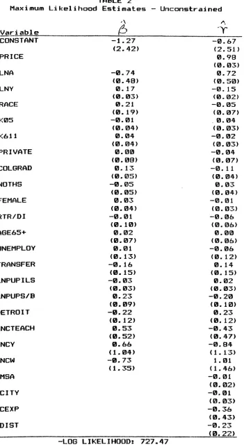
(13)The full information maximum likelihood estimates of the parameters of equation (13) are given in Table 2. Estimates of
fi are in column 1 and estimates of y are in column 2.
While the primary purpose of this effort is to provide prediction equations to be used
positive and the estimated effect of expenditure on marginal rate of substitution was sig-nificantly negative. The implied income elasticity of demand based on these estimates is .23. The implied price elasticity of demand is -.87.2
The reader is free to explore and interpret other coefficients that appear in the table. The estimates of
yt
and "A (where yA is the element in the vector 'Yx that is associated with in A) tell us about the correlation between e and (t, X), which is to say, the importance of Tiebout sorting. As we demonstrate in the appendix, if there were no correlation betweene and (t, X), then -y, and 7A would both be zero. We find, using asymptotic t-tests, that
both of these coefficients are significantly different from zero at the 1% level.
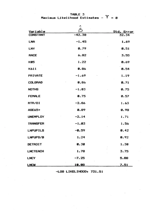
In Table 3 we present the maximum likelihood estimates of the marginal rate of sU)sti-tution function where no correction for Tiebout sorting is made. These estimates constrain e to be uncorrelated with w1 and w2, the unobserved determinants of tax price and actual
expenditures (that is, yt and yx are constrained to zero). Almost all the coefficients of the constrained model are substantially larger than those of the general model. The likelihood ratio test between the constrained and unconstrained models yields a Chi-square(2df) of 8.10. As a result, the hypothesis of zero covariance, or the exogeneity of both expenditures and tax price, can be rejected at the 1% level.
4. Testing for Efficiency of Community Expenditures
Predicting Community Sums of Marginal Rates of Substitution
Now that we have prediction equations for individual marginal rates of substitution, we can use these equations, together with information available from the Census about the distributions of economic and demographic characteristics in school districts, to predict
the sum of marginal rates of substitution in any school district in Michigan. The way we proceed is as follows. Let Si be the set of households in community
j
and let mi =ZiEs;
mi.
Since Equation (13) is linear in t, X, and W, we can estimate the sum of marginal rates of substitution as follows:9 =
Z
mi = $t' + (/' +' ')X + - WI (14)ies;
where ti = ZiES ti, Xi = lEs X; and W = Wjj
1.
If we sum the expression in Equation (3) over all consumers in community
j,
we havemi = m; = #'X'
+
E&(15)iES,
2 'These estimates are obtained b~y solving the equation m = 1 In A
+#/2
in Y + constants for in A as a function of the other variables. When a consumer is getting the desired arnount of public goods, mf is equal to the price p that he pays for them. Then we have ini A = (p -#g2 hii Y 4constants)/p3i. The income elasticity is therefore just -#32/1 and the price elasticity evaluated at the mean price is just pi//A. Usingwhere e' = i e. From adding the expressions in Equation 11, it follows that
E(e'1jt,1X', W')
= 'yt t+'yX'
+ yy4W' .
(16)
From Equations (14), (15), and (16) it follows that:
t' -i- =
(#'
-fp'+E
-y'XX+(i( -3g)t' +(
Y)Wo, -y'
- e +E(E It',X', W'). (17)
For each community, we must find the aggregate vectors, Xj, and W'. Most of the components of these vectors are aggregates that are readily available in statistics published by the U.S. Census or the Michigan Department of Education. For example the census records the number of households in each community, the number of persons over 65 years of age and the number of persons with a college education.
Calculating the sum of In Y in each community is slightly more difficult. Here the problem is twofold: the Census reports information on income rather than log of income, and the form of the information differs between families and unrelated individuals. The approach we have taken is to estimate the mean of in Y for families from the information available on family income and the mean of In Y for individuals from the information on individual income. Weighting these by the number of families and the number of unrelated individuals, respectively, we obtain the district-wide mean of ln Y. The distribution of families in a school district was given for fifteen income brackets, allowing us to estimate the median family income (we assume a uniform distribution within each bracket). Then assuming income is distributed log-normally, we have, for families,
mean(ln Y)
=median(ln Y)
=in median(Y).
For unrelated individuals, the only data available were aggregate income and the number of individuals. For them we took in mean(Y) as an approximation for mfean(ln1 Y).
Efficiency
in the Interest of Society as a WholeLet cj be the marginal cost of providing the local public good to community
j.
Then the Samuelson efficiency condition for communityj
is expressed by the equationcj = m' =
m;=3'X' +.e'.
(18)
iESj
In our application the public good is per student expenditures in the local public schools.
The cost to a school district of increasing expenditures per student by one dollar is equal
to the number of students in the district. Therefore c
1is
just
the number of students
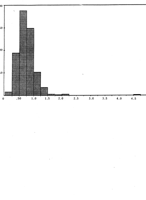
The distribution of the computed values of the ratio of community mrs to marginal cost is shown in Figure 1. More than 80% of the school districts have riii/c, < 1.
It is possible to use our estimates to identify school districts for which there is an especially large divergence between the sum of marginal rates of substitution and marginal cost. But it is important to remember that for a
Particular
community, such a divergence is n9t necessarily an indication of inefficiency. It might be that unobserved differences in tastes for education or unobserved cost differences account for the discrepancy. In our notation, this would mean that E3 differs from its expected value.Although e0 - E(e jIts, X', Wi) will vary across individual districts, we can expect
that the average value of this difference over the 497 school districts in Michigan will
be
very close to zero. To test for a systematic tendency for overspending or underspending in Michigan, we therefore want to study the average over all Michigan school districts of the ratio rhn/cy. Under the null hypothesis that there is no systematic bias toward overspending or underspending, we would have 1nj>
'1z'= 1. From Equation (17) it follows thatn._ c_
=1
where X = 1 "='" - W = n w and = .- gXW)
nj= =1 c" j1 1c nEj c)
The variance of the expression in Equation (19) comes from two sources. One source is the variance of the fl's and j's around the "true" /3's and -y's. The second source of variance is the random variable E. Since E is a mean of statistically independent community specific random variables taken from 497 communities, the latter source of variance can reasonably be neglected. As we see from Equation (19), the difference i i- 1 is a linear combination of the difference between our parameter estimates for the fl's and -y's and their expected value. Since we have estimates of the variance-covariance matrix for these estimates, we can readily calculate an estimate of the standard deviation of the expression in Equation (19). According to our computations, the random variable 1
ZEn
m' takes the value .748 and the estimated standard error of this random variable is .09. Therefore we must reject the hypothesis of efficiency at the 95% significance level.These results suggest that the sum of marginal rates of substitution between local public education and other goods in Michigan communities tends to be less than the marginal cost of public goods. If the only beneficiaries of local public education are the residents of the community in which the education is provided, this would mean that most communities spend too much on local public education from the standpoint of social efficiency.
Efficiency in the Interest of the Localities.
local public education, we might compare this sum with the fraction of marginal costs that are borne by the voters in the school district. This would give us a test of whether school districts are acting efficiently in the interest of their own residents.
In Michigan, at the time of this survey, marginal increments to local revenue came from the local property tax. In most school districts a large fraction of the property tax
base is non-residential property and, of course, much of this property is either not locally
owned or concentrated in the hands of a very small number of voters. (For the included communities non-residential property is 35% of the property tax base.) If people believe that taxes assessed on non-residential property are fully exported and if the fraction of the local property tax base that is residential property is s3, then efficiency from a purely local point of view requires that m/cj = s1.
For 454 of the 497 communities that we observed, - - si is positive and for the remaining communities ' - si is negative. Under the null hypothesis that, on average,
= si, Equation (19) would be replaced by
-
-
-
=
('
+P '^7)
+ ($7
t)^t+(7'
-7)W+(20)
j=1where 3= n
1Si.
As it turns out, s"= .649 and n_,1 = .748. The estimated standard error of the
random variable - is .09. Therefore we are not able to reject the hypothesis
that, on average, - . = si.
5. Concluding Remarks.
This is, as far as we know, the first attempt in the literature to empirically test the
Samuelson conditions for efficient provision of public goods. Accordingly, we urge the readers to interpret our results cautiously. Other data sources and other methods of approach may lead to very different conclusions. To illustrate this point, we must point out that our corrections for Tiebout bias had a very strong effect on our results. If we
estimate the marginal rate of substitution functions, making no correction for Tiebout
bias, but otherwise pursuing the same methods, we find that the average value of the ratio of summed marginal rates of substitution to marginal cost in Michigan school districts is 1.62 while with the correction, the average value is 0.748. Thus the uncorrected estimates
would suggest substantial underspending and the corrected estimates suggest a tendency
toward overspending.
resulting efficiency calculation is .80, much closer to the result of applying the endogeneity correction to both variables.
These facts suggest that if someone wants to prove either that too much or too little is
being spent, he can find the desired result by fiddling with the specification of the model.
We think that the correction we have chosen is preferable on theoretical grounds to the
uncorrected estimates. Other data sets and other choices of instrumental variables may lead to different conclusions. But if there is a strong tendency in one direction or another, we expect that it would be confirmed in repeated studies. We hope that others will try to investigate this question empirically.
With these qualifications in mind, suppose we take our empirical results as roughly
correct, what conclusions could we draw? On average it appears that the sum of marginal rates of substitution for local public education is lower than marginal cost. If there are no
spillovers of benefits from one school district to others, this would mean that local school districts are overspending from the standpoint of social efficiency. But, on average, the
sum of the residents' marginal rates of substitution is about equal to the share of the costs
that are borne by local taxpayers. This means that local school districts tend to act quite efficiently in promoting the interests of the voting population which does not bear the entire cost of local education. Whether this is a socially efficient arrangement depends on the size of the externalities generated by local education for the rest of the economy.
Appendix
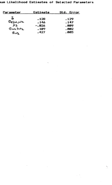
The system of equations 3, 8, and 9 in the text is assumed to have a vector of random disturbances (e, wi ,w2) with a joint normal distribution with mean zero and with off-diagonal covariances that are not necessarily zero. It is the fact that these off-off-diagonal terms, owl,, cw2, and aw1 w2 are non-zero that causes Tiebout bias to be a problem.
A full information maximum likelihood procedure is used to obtain consistent parameter estimates. Letting R represent an individual's more/same/less response, the likelihood function that is maximized represents the joint probability of observing the given set of
(R, t, ln A) vectors. For example, given
X
0
andWo,
the likelihood of observing a "more" response, tax price to, and expenditure level, Ao is:pr(more, to,in Ao)
=If(e,
wo, w
2o)de
to ta--pXo
where w
1
= to - 6111o - 91 2Wo and w20 = In Ao - 021Io - 62 2W0. Using Bayes' law,f(e,wi, w
2)
=f(EIt,w
2)f(wi,w
2)
=f(eIwi,w
2)f(wmI
2)f(w
2).
And, from standard results for conditional distributions of multivariate normal variables, E(Ejwio, w2o) = Aiw10 + \ 2w2 0 and E(wiolw2o) = A3w2 0 where
2
to -# -
Xo+
W
1
E0 io - m2 1 2In - w1+l (I 22 2W22
2 2
Wi w2 W1lW2
and
Then the term in the likelihood function corresponding to this observation is
(we- - 1 2)
(2i0 - Asw o 2
w22
In a similar fashion, the likelihood function for the entire sample becomes
L = In F t #X -6-hu-k2
iELess ln EW1A,w2
+
In F t -
p'Xi
+
6-Aiw 2w2F
t- X-6-
AW 1 A2w2iE-SaFme o|ww,2 w2 22)))
+ -
F
(t 1 -IJIXi+±6-
li- A2W2 :)+
In
1 - F A--eiE More 0 (I 1 2lw
n 2(wu
1 -A 3 2i)2 ii
-
t(ln
27rcT1 I 2+
In 27r22) - 2 2 Z-Substituting w12 = ti - 61X; - 012Wi and w2i = in
A
-621Xi) - 022W , we maximizethis function with respect to
fi,
6, 8, A1, A2, A3,0eWi,w
2,W2,W1 , and uw2.We are concerned here, however, with predicting marginal rates of substitution, rather than with estimates of the structural model. That is, we are concerned with
m = 3'X +
A
1(t - 8n1XC-- 91 2W) + A2(lnA - 02X -022W).
Gathering terms and making obvious substitutions, we can write
ml = -'X±+ ygt t'7X + 'wW.
These are the reduced form parameter estimates
fi
and y that are reported in Table 2. Notice that 7Yt = Al and 7A = A2. Some of the other parameter estimates are reported inReferences
Barlow, R. (1970) "Efficiency Aspects of Local School Finance," Journal of Political
Econ-omy, 78, 1028-1039.
Bergstrom, T. (1979) "When Does Majority Rule Supply Public Goods Efficiently?,"
Scan-dinavian Journal of Economics, 8, 216-227.
Bergstrom, T., D. Rubinfeld and P. Shapiro (1982) "Micro-Based Estimates of Demand Functions for Local School Expenditures," Econometrica, 50, 1183-1205.
Bewley, T. (1981) "A Critique of Tiebout's Theory of Local Public Expenditures," Econo-metrica, 49, 713-737.
Bowen, H. (1943) "The Interpretation of voting in the Allocation of Economic Resources,"
Quarterly Journal of Economics, 58, 27-48.
Brazer, H. (1961) "Some Fiscal Implications of Metropolitanism," in Metropolitan Issues:
Social, Governmental, Fiscal, ed. G. Birkhead. Syracuse, New York: Maxwell
Gradu-ate School of Public Affairs, Syracuse University.
Brennan, G. and Buchanan, J. (1980) The Power to Tax: Analytical Foundations of a Fiscal Constitution.: .
Courant, P., Gramlich and D. Rubinfeld (1979) "Public Employee Market Power and the Level of Government Spending," American Economic Review, 69, 806-817.
Denzau, A., R. MacKay and C. Weaver (1981) "On the Initiative Referendum Option and the Control of Monopoly Government," in Tax and Expenditure Limitation, ed. H. F. Ladd and T. N. Tidernan. Washington, D.C.: Urban Institute, 191-222.
Downs, A. (1960) "Why the Government Budget is Too Small in a Democracy," World Politics, 12, 541-563.
Galbraith, J. K. (1958)
TheAffluent
Society.Cambridge, Mass.: Houghton-Miflin.
Goldstein, G. S. and M. V. Pauly (1981) "Tiebout Bias and the Demand for Local Public
Goods," Journal of Public Economics, 16, 536-550.
Gramlich, E. and D. Rubinfeld (1982) "Using Micro Data to Estimate Public Spending Demand Functions and Test the Tiebout and Median Voter Hypothesis," Journal of
Political Economy, 90, 535-560.
Heckman, J. (1979) "Sample Selection Bias as a Specification Error," Econometrica, 47,
153-161.
Inman, R. (1982) "Wages, Pensions, and Employment in the Local Public Sector," in Public Sector Labor Markets, ed. P. Mieszkowski and G. Peterson. Washington, D.C.: Urban Institute, 110-118.
Ladd, H. (1975) "Local Education Expenditures, Fiscal Capacity, and the Composition of
Property Tax Base," National Tax Journal, 28, 145-150.
Romer, T. and Rosenthal, H. (1978) "Political Resource Allocation, Controlled Agencies and the Status Quo," Public Choice, 33, 4, 27-43.
Rubinfeld, D., P. Shapiro and J. Roberts (1987) "Tiebout Bias and the Demand for Public Goods," Review of Economics and Statistics, 69, .
Samuelson, P. A. (1954) "The Pure Theory of Public Expenditure," Review of Economics
and Statistics, 26, 387-398.
Shapiro, P., and Sonstelie, J. (1982) "Did Proposition 13 Slay Leviathan?," American Economic Review, 72, 184-190.
Stiglitz, J. (1982) "The Theory of Local Public Goods Twenty-five Years after Tiebout: A Perspective," NBER Working Paper no.954.
Tiebout, C (1956) "A Pure Theory of Local Expenditures," Journal of Political Economy, 64, 416-424.
Weisbrod, B. (1964) External Benefits of Public Education: An Economic Analysis. Prince-ton, N.J.: Princeton University, Industrial Relations Section.
Williams, A. (1966) "The Optimal Provision of Public Goods in a System of Local Gov-ernment," Journal of Political Economy, 74, 10-33.
TABLE 1
Definition of Variables
PR ICLE
LNA
LNY
BLACK
K05 1(61 1
PR
TATEI
COLGRAD MOTHS FEMALE RTR/DI AGE65+ UNEMPLOY TRANSFER LNPUPILS LNPUPS/B DETROIT LNCTEACH LNCY LNCW SMSA CCITY PCEXP YDIST
Individual 's tax price
Log of actual per pupil school expenditures
Log of household disposable income
Dummy variable: 1 if black, 0 otherwise
Number of children younger than six years old
Number of children aged six to eleven
Dummy variable:
otherwise
Dummy variable:
Dummy variable:
0 otherwise
1 if child in private school, 0
if a college graduate, 0 otherwise
if did not graduate from high school, 1
1
Dummy variable: 1
Dummy variable: 1
Dummy variable: 1
Dummy variable: 1
Dummy variable:
otherwise if if if if I
female, 0 otherwise
retired or disables, 0 otherwise
over age 65, 0 otherwise
unemployed, 0 otherwise
if receives transfer payments, 0
Log of total school district enrollment
Log of number of students per school
Dummy variable: 1 if resident of Detroit, 0 otherwise
Log of county average teachers' salary
Log of county average income
Log of county average wage rate
Dummy variable: I if in SMSA, 0 otherwise
Dummy variable: 1 if in central city,
@
otherwisePercent change in school district expenditures per
pupil over the previous year
[image:21.608.46.551.43.750.2]TABLE 2
Maximum Likelihood Estimates - Unconstrained
Variable CONSTANT PRICE LNA LNY RACE K05 K611 PRIVATE COLGRAD NOTHS FEMALE RTR/DI AGE65+ UNEMPLOY TRANSFER LNPUPILS LNPUPS/B DETROIT LNCTEACH LNCY LNCW -1.27 (2.42) -0.74 (0.48)
0.17
(0.03) 0.21(0. 19) -0.01 (0.04) 0.04 (0.04) 0.00 (0.08) 0.13 (0.05) -0.05 (0.05) 0.03 (0.04) -0.01 (0. 10) 0.02 (0.07) 0.01 (0.13) -0. 16 (0.15) -0.03 (0.03) 0.23 (0.09) -0.22 (0.12) 0.53 (0.52) 0.66 (1.04) -0.73 (1.35) -0.67 (2.51) 0.98 (0.03) 0.72 (0.50) -0.15 (0.02) -0.05 (0.07) .0.04 (0.03) -0.02 (0.03) -0.04 (0.07) -0.11 (0.04) 0.03 (0.04) -0.01 (0.03) -0.06 (0.06) 0.00 (0.06) -0.06
(0. 12)
0.14 (0.15) 0.02 (0.03) -0.20 (0.10) 0.23
(0. 12)
-0.43 (0.47) -0.84 (1.13) 1.01 (1.46) -0.01 (0.02) -0.01 (0.03) -0.36 (0B.43) -0.23
(0. 22)
SMSA
CCITY
PCEXP YDIST
[image:22.612.140.491.88.732.2]TABLE 3
Maximum Likelihood Estimates -0
Variable CONSTANT LNA LNY RACE K05 K611 PRIVATE COLGRAD NOTHS FEMALE RTR/DI AGE65+ UNEMPLOY TRANSFER LNPUPILS LNPUPS/B DETROIT LNCTEACH LNCY LNCW -42.38 -1.45 0.79 6.82 1.22 0.86 -1.69 0.86 -1.03 0.75 -2.86 0.89 -2.14 -1.03 -0.59 1.24 0.30 1.78 -7.25 10.08
-LOG LIKELIHOOD:
Std. Error
32.34 1.69 0.51 3.55 0.69 0.54 1.19 0.71 0.75 0.57 1.63 0.98 1.71 1.56
0. 42
0.92 1.30 3.75 5.88 7.51 r
now w wr or r
[image:23.612.55.562.47.773.2]flax i mum Likelihood
Parameter
c.YW. 1OL
TABLE Al
Estimates of Selected Parameters
Estimate
Std.Error
.128 .129
.146 .147
-. 026 .0
.109
.0
[image:24.611.147.535.101.740.2]FIGURE
1-COMMUNITY MARGINAL RATES OF SUBSTITUTION
200
150
100
[image:25.608.42.540.75.755.2]Recent Crest Working Papers
87--1: Jeffrey K. MacKie-Mason, "Nonlinear Taxation of Risky Assets and Investment, With Application to
Mining" September, 1984.
87-2: Jeffrey K. MacKie-Mason, "Sequential Decision Problems and Asymmetric Information" September, 1985.
87-3: Michelle J. White, "Contract Breach and Contract Discharge due to Impossibility: A Unified Theory"
July 29, 1987.
87-4: Ted Bergstrom, "Systems of Benevolent Utility Interdependence" May 19, 1987.
87-5: Ted Bergstrom, "A Fresh Look at the Rotten Kid Theorem-and Other Household Mysteries"
Novem-ber, 1986.
87-6: Michelle J. White, "The Corporate Bankruptcy Decision" July, 1987.
87-7: Michelle J. White, "Location Choice and Commuting Behavior in Cities with DecentralizedEmploy-ment" July, 1987.
87-8: Lawrence E. Blume David Easley, "Implementation of Walrasian Expectations Equilibria" December,
1985.
87-9: Lawrence E. Blume, "Lexiocographic Refinements of Nash Equilibrium" April, 1986.
87-10: David Lam, "Lorenz Curves, Inequality, and Social Welfare Under Changing Population Composition"
June 16, 1987.
87-11: Mark Bagnoli, Naveen Khanna, "Equilibrium with Debt and EquityFinancing of New Projects: Why More Equity Financing Occurs When Stock Prices are High" June, 1987.
87-12: Mark Bagnoli, Barton L. Lipman, "Provision of Public Goods: Fully Implementing the Core through
Private Contributions" March, 1987.
87-13: Mark Bagnoli, Barton L. Lipman, "Successful Takeovers without Exclusion" August, 1987.
87-14: Mark Bagnoli, Michael McKee, "Controlling the Game: Political Sponsors and Bureaus" May, 1987.
87-15: Mark Bagnoli, Michael McKee, "Can the Private Provision of Public Goods be Efficient?-Some
Experimental Evidence" March, 1987.
87-16: Mark Bagnoli, "Non-Market Clearing Prices in a Dynamic Oligopoly with Incomplete Information"
January, 1986.
87-17: John Laitner, "Bequests, Gifts, and Social Security" February 28, 1986.
87-18: John Laitner, "Dynamic Determinacy and the Existence of Sunspot Equilibria" May 12, 1986.
87-19: David Lam, "Does a Uniform Age Distribution Minimize Lifetime Wages?" August 12, 1987.
87-20: David Lam, "Assortative Mating with Household Public Goods" April, 1987.
87-21: Jeffrey A. Miron, Stephen P. Zeldes, "Production, Sales, and the Change in Inventories: An Identity that Doesn't Add Up" June 1987.
87-22: Jeffrey A. Miron, Stephen P. Zeldes, "Seasonality, Cost Shocks, and the Production Smoothing Model of Inventories" December, 1986.
87-23: Hal R. Varian, "Differences of Opinion in Financial Markets" March, 1985.
87-24: Roger H. Gordon, Hal R. Varian, "Taxation of Asset Income in the Presence of a World Securities
Market" August, 1986.
87-25: Hal R. Varian, "Measuring the Deadweight Costs of DUP and Rent Seeking Activities" November, 1982.
87-26: Hal R. Varian, "Price Discrimination" January, 1987.
87-29: hal R. Varian, "Optimal Tariffs and Financial Assets" April, 1987.
87-30: Jonathan Cave, Stephen W. Salant, "Cartels That Vote: Agricultural MarketingBoards and Induced
Voting Behavior" August, 1987.
87-31: Stephen W. Salant, Donald I. Negri, "Pastures of Plenty: When is the Standard Analysis of Common
Property Extraction Under Free Access Incorrect?" July 10, 1987.
87-32: Stephen W. Salant, "When is Inducing Self-Selection Sub-optimal for a Monopolist?" February, 1987.
87-33: Stephen W. Salant, "Treble Damage Awards in Private Lawsuits for Price-Fixing" August, 1987.
87-34: Stephen W. Salant, Roy Danchick, "Air Force Academy Attrition: A New Perspective on the College
Dropout Problem" August, 1987.
87-35: Stephen W. Salant, Eban Goodstein, "Committee Voting Under Alternative Procedures and
Prefer-ences: An Experimental Analysis" April 20, 1987.
87-36: Robert B. Barsky, Jeffrey A. Miron, "The Seasonal Cycle and the Business Cycle" June, 1987.
87-37: Robert B. Barsky, N. Gregory Mankiw, Jeffrey A. Miron and David N. Weil, "The Worldwide Change in the Behavior of Interest Rates and Prices in 1914" July, 1987.
87-38: Jeffrey K. MacKie-Mason, "Taxes, Information and Corporate Financing Choices" April, 1986.
87-39: Avery Katz, "The Effect of Frivolous Lawsuits on the Settlement of Litigation" August, 1987.
88-1: Carol A. Jones, Suzanne Scotchmer, "The Social Cost of Uniform Regulatory Standards in a Hierar-chical Government" December, 1987.
88-2: Ted Bergstrom, Judy Roberts, Dan Rubinfeld, Perry Shapiro, "A Test for Efficiency in the Supply of Public Education" December 12, 1987.
88-3: Mark Bagnoli, J. Bradley Barbeau, "Competition and Product Line Choice" February, 1988.
88-4: Severin Borenstein, Paul N. Courant, "How to Carve a Medical Degree: Human Capital Assets in Divorce Settlements" December, 1987.
88-5: Mark Bagnoli, Stephen W. Salant, Joseph E. Swierzbinski, "Pacman Refutes the Coase Conjecture: Durable-Goods Monopoly with Discrete Demand" January, 1988.
88-6: Jonathan Cave, Stephen W. Salant, "A Median Choice Theorem" December 29, 1987.
88-7: Mark Bagnoli, Naveen Khanna, "Why Are Buyers Represented by Seller's Agents When Buying a House?" December, 1987.
88-8: Mark Bagnoli, Roger Gordon, Barton L. Lipman, "Takeover Bids, Defensive Stock Repurchases, and
the Efficient Allocation of Corporate Control" October, 1987.
88-9: Mark Bagnoli, Barton L. Lipman, "Private Provision of Public Goods can be Efficient" November, 1987.
88-10: Michelle J. White, "Urban Commuting Journeys are Not "Wasteful"" February, 1988.
88-11: Avery Katz, "A Note on Optimal Contract Damages When Litigation is Costly" February, 1988.
88-12: Ted Bergstrom, Jeff MacKie-Mason, "Notes on Peak Load Pricing" February, 1988.
88-13: Jerry A. Hausman, Jeffrey K. MacKie-Mason, "Price Discrimination and Patent Policy" February,
DeptE
33ergst
c m,
Ted
ttc."--A
Test .?or ficiency
1n. the
Saxp1ly af
Public
TITLE