An Improved Differential Evolution Algorithm Using Adaptive Multiple Mutation Strategies for the Economic Load Dispatch Problems

2018 International Conference on Computational, Modeling, Simulation and Mathematical Statistics (CMSMS 2018) ISBN: 978-1-60595-562-9

An Improved Differential Evolution Algorithm Using Adaptive Multiple

Mutation Strategies for the Economic Load Dispatch Problems

Qiang ZHANG

1,2,*

_{, De-xuan ZOU}

1

_{, Xin SHEN}

1

_{and Peng XIAO}

1

1_{College of Electrical Engineering and Automation, Jiangsu Normal University,}

Xuzhou Jiangsu 221116, China

2_{College of Information and Electrical Engineering, Xuzhou Open University,} Xuzhou Jiangsu 221000, China

*Corresponding author

Keywords: Improved differential evolution, Economic load dispatch, Mutation, Modified repair

process, Equality constraint.

Abstract. An improved differential evolution algorithm using adaptive multiple mutation strategies (IMMSDE) is proposed to solve the economic load dispatch (ELD) problems with or without valve-point effects (VPE). Unlike classical differential evolution (DE) algorithm, three mutation strategies and five adaptive parameters participate in the IMMSDE. A mutation strategy is randomly selected from the strategy pool in order to enlarge the search range, which is beneficial for preventing the solutions from falling into location optima. On the other hand, the adaptive parameters with learning ability improve the search accuracy and the speed of convergence. Additionally, a repair method is used to handle equality constraints, which enables IMMSDE to find feasible solutions rapidly. Four ELD cases are selected to testify the effectiveness of four DE algorithms on solving ELD problems. Results show that IMMSDE performs better than the other algorithms for the ELD problems and can always find the solutions satisfying the equality constraints.

Introduction

Economic load dispatch (ELD) [1] is important for improving the economic efficiency and stability of power systems. The goal of ELD is to minimize the cost of power generation under the conditions of meeting the load demand and operational constraints. However, due to the existence of the valve point effect of the thermal power unit, the unit's power consumption characteristic function is a non-differential nonlinear function. At the same time, due to the constraints of the transmission system, power system stability and other conditions, the feasible domain of the ELD problem is non-convex. In short, the economic load distribution of the power system is a complex optimization problem with high dimensionality, nonlinearity, non-differentiability, and multi-constraint.

The original ELD problems can be solved by classical mathematical methods [1-3], such as micro-increment method, quadratic programming and nonlinear programming, since the quadratic functions are used as the cost functions which are differentiable. However, these approaches can hardly work for the ELD problems with additional considerations as the quadratic functions are no longer suitable for characterizing these ELD problems.

Differential evolution algorithm (DE) was firstly proposed by Price and Storn, in 1995. DE is simple in principle, and thus it is easy to understand and implement. It is one of the most effective stochastic optimization algorithms. Due to these merits, it has been applied into more and more practical optimization problems. There are four cases of ELD problems studied, which reveal good performance of the improved DE. Three mutation strategies are cooperated to improve the performance of the algorithm, and an adaptive parameter setting method is used in the mutation factor, crossover factor and disturbance factor.

In light of the above studies, the IMMSDE is proposed to solve the ELD problems without valve-point effects (VPE) [1,567] and the ones associated with VPE. There is a folds in our contributions, an improved DE algorithm is proposed to further enhance the performance of the original DE algorithm.

Mathematical Model of Economic Load Dispatch Problems

The Objective Function

The goal of ELD is to minimize the total fuel cost under the constraints of a power system. Two types of ELD problems are studied in this paper: one without VPE and the other one with VPE. As the turbine intake valve suddenly opens, wire drawing will occur, and a pulsating effect will be added to the unit's consumption characteristic curve to generate a valve point effect. Studies have shown that ignoring the valve point effect will significantly affect the solution accuracy, their objective functions are expressed as follows [9-11]:

   2 

1 1

min N i i N i i i i i

i i

F P a P b P c

 

  





(1)

 



2



 min 





1 1

min N i i N i i i i i+ isin i i i

i i

F P a P b P c e f P P

 

   





(2) Here, N is the total number of generators in the power system. Fi(orFi) stands for the fuel cost of

the generators unity i (in $/h); a_ib_iandc_i stand for the cost coefficients of generator i; e_i and f_i stand

for the valve-point loading coefficients of generator i; Pi stands for the generating power of

generator i (in MW);

Constraints

There are two constraints in the ELD problems. One is inequality constraint, and the other is equality constraint, they can be formulated by [8-10]:

1

N

i L D i

P P P



 



(3)

min max

i i i

P  P P (4)

Equation (3) is an equality constraint considering power balance, and it requires that the power generation is equal to the sum of total demand (PD) and total transmission line loss (PL).

Equation (4) is an inequality constraint, and it requires that the power of every generator lies between the lower bounds ( min

P ) and upper ( max

P ) bounds. When the power system is densely covered,

we can ignore the network loss. For the cases studied here, the transmission losses PL is excluded,

hence (4) can be reformulated as follows:

1

N i D i

P P 





(5) (4) is easy to meet, for example, if the variable Pi exceeds the boundary, it will be set to the exceeded

First, the penalty function, second, the remaining one-dimensional variables is determined by equality constraint, after N-1 dimensional variables had finished search, but A larger number of invalid solutions will be generated and reduce the diversity and convergence speed, resulting in the inability to find a global optimal solution. In [11], a repair process was used to each solution to cope with equality constraints. In the modified repair process, the j

i

x represents the ith i1,2,...,nvariable

in the j th j1,2,...,Np individual solution j i

x ,therefore,  1, ,...,2   1, ,...,2 

j j j

n n

P P P  x x x a component j

i x is

selected randomly and checked to see whether it reaches the low bound min

P (upper bound max

P ) if the

sum of all Piis larger(smaller) than PD. If it does, this component is considered to be undesirable

and will be exclude from the candidate vector. Meantime, a new component will be randomly selected from vector which does not include the previous eliminated components. This process is repeated until a new component which is unequal to its low (or upper) is found. This operation is necessary, because it can avoid many ineffective repairing trials which do not play any positive role in reducing constraint violations.

After the repair process, the penalty function method is adopted, which is formulated by:

 

1

N i i i

f F P w







 (6)

 

1

N i i i

f F P w







 (7)

Equation (6) is the ELD problems without VPE, and (7) is the ELD problems with VPE. Here, w

that represents the constraint violations of the equality is formulated by

1

N i D i

w P P







 , and  is positive

penalty factor. In this paper, a repair method is presented, which is combined with penalty method to solve the equality constraints.

Differential Evolution Algorithm and Its Four Variants

The DE algorithm is a self-organization minimization method based on group evolution. The main idea is to introduce a new differential variation model that can use the individual differences in the current population to construct variant individuals. Compared with traditional evolutionary algorithms, differential variation mode is the unique evolutionary operation in the DE algorithm. The following is a brief introduction to the evolution of the classic DE algorithm.

The Procedure of the Classical DE Algorithm

Step 1: Initialization. The Np vectors with Nd dimension are adopted in the DE, and they are

initialized randomly from a uniform distribution as follows

 

min max min

ij i i i

X X  X X rand (8)

Here rand stand for a randomly number between 0 and 1. Additionally, DE parameters are

initialized in this step, and these parameters include mutation factorF, crossover rateCR, population

size Np and the maximal iteration numberNi.

 Step 2: Mutation operation. For current population, each new mutation vector is given by:

 

1

3 1 2

k k k k

i i i i

v x F x x (9)

Here, k1

i

v denotes the mutant vector of the ith vector at the current k1th generation, The vector

1

k i x , 2

k i x , 3

k i

x are selected randomly from the current population, which keep different from each other.

 Step 3: Crossover operation. The crossover operation generates the trail individual. A new trail vector k1

i

u is generated by discrete crossover operation between

k i

v _and vik 1



1

1~ 1 , if rand < CR or j =

, otherwise k ij d k i k ij v r u x     

 (10)

Here, r1~dis random integer in the range  1,D , CR 0,1 .

 Step 4: Selection operation. Greedy selection algorithm is adopted in the DE, and each trail vector k1

i

x is expressed as:

   

1 1

1 , if

, otherwise

k k k

i i i

k

i k

i

u f u f x

x x

 

 _{ } 

 (11)  Here f x  is objective function, if  1

k i

f u is smaller (or better)  k i f x , k1

i

u form crossover

operator assigned to k1

i

x , otherwise, k i

x is assigned to k1

i x.

 Step 5: Judge stopping condition. If the theoretical optimal value or maximum number of iterations Ni is reached, computation is stopped. Otherwise, Steps 3 and 4 are repeated.

Factors Affecting the Performance of Differential Evolution Algorithms In this paper, three mutation strategy are proposed.

 Strategy 1:





1

elite_ 1 2

k k k k k k

i i best i i i

v x F x x x x (12)

 Strategy 2:

 

1

1 2

k k k k

i best i i

v x F x x (13)

 Strategy 3:

 

1

3 1 2

k k k k

i i i i

v x F x x (14)

Here, elite_

k best

x denotes the best solution in population which selected randomly from eNp vector

particles in all vector particles at kth generation. after testing, it is best choice thatpis given by 0.2

for the ELD. k best

x is the best solution in all the population.

The one of three strategies are selected by two threshold T1andT2,R1R2is both a random which is

in the range[0,1]. If R1 is smaller than T1and R2 is smaller than T2too, the strategy 1 is selected; if R1

is smaller thanT1, but R2 is larger thanT2, the strategy 2 is selected; otherwise, the strategy 3 is

selected.

In order to make IMMSDE self-adapting, The definition of F, CR is based on previous generation

of result ,if the value of objective function in the current generation is superior to previous one, the value of F, CR is inherited in next generation, otherwise, they is given by the mean value of F, CR

from all vectors. In addition, if the first vector in the population is larger than the mean value of the entire vectors, the former is replaced by the later in the each iteration.

The Procedure of the Proposed Algorithm

 Step 1: Parameter settings. Population sizeNp, vector dimension Nd , the maximal iteration

numberNi.

0.1,0.8

F ;CR0.3,1;T10.95;T =0.992 ; e=0.2.

 Step 2: Initialize variables. F, CR and



X X,



are randomly initialized within the specified

range.

 Step 3: Mutation operation.

 Step 4: Crossover operation.

 Step 6: Generate new parameter. According to the comparison results in the selection operation, the winning vector particles are found and the corresponding parameters used are recorded

 Step 7: Judge stopping condition. If the theoretical optimal value or maximum number of iterations is reached, computation is stopped. Otherwise, steps 3 and 6 are repeated.

Experimental Results and Analysis

In this section, four cases are selected to testify to the better performance of IMMSDE comparing other three DE variants on solving the ELD problems. The parameters of all cases are provided in corresponding literatures. Two cases are the ELD problems without VPE: 6-unit [11], 38-unit [12, 14]. The other two cases are the ELD problems associated with VPE: 3-unit case (Pd850 MW) [1,

13], and 13-unit case (Pd2520 MW) [8].

The parameter settings of three comparing DE variants are provided in the literatures [16-18] too, it is no necessary to describe them again. To assure a fair comparison, the population size Np is set

to 40 for all the four DE approaches. As the complexity of the case increases, the maximum allowable generation Gmax also increases, but the four compare algorithms are set to the same Gmax in each case. In the penalty method, the penalty coefficient  is set to 1e20.In addition, Matlab language is used for simulate experiments under the environment of an Intel Core i5 [email protected] GHz. The optimization results of 30 independent runs are summarized in Table I.

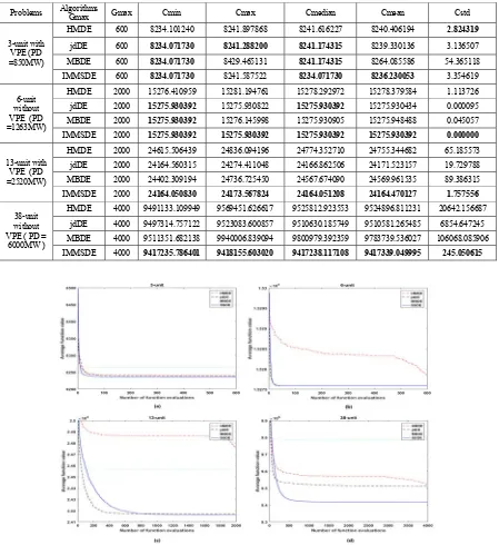
In Table 1, the terms “Cmin”, “Cmax”, “Cmedian” and “Cmean” denote the minimal, maximal, median and mean value of 30 results, respectively. Cstd stands for the standard deviation of 30 objective function values. In the meantime, the Cmean is also superior to those of the other four performances, Followed by Cstd. For 3-unit with VPE case, the Cmean value of IMMSDE is smallest, Cmin, Cmedian value is the same to HMDE and MBDE. With regard to 6-unit without VPE case, the Cmax,Cmean and Cstd value is respectively smallest, To 13-unit with VPE case, the Cmin, Cmax and Cmean value of IMMSDE are superior to those of the other three approaches, meanwhile, IMMSDE can find relatively best Cmedian value and best Cstd value. For 38-unit without VPE case, IMMSDE get overall better than other approaches in each performance. It highlights the advantages of IMMSDE on the solution of complex problem

The average convergence curves of HMDE, jdDE, MBDE, and IMMSDE are plotted in Figure 1 for four ELD cases. We can find intuitively that IMMSDE convergence finally achieves lower than other three algorithm for 3-unit case with VPE, 6-unit case and 38-unit case without VPE. On the other hand, in the 13-unit case with VPE, IMMSDE is obviously better than HMDE and MBDE but slightly better than jdDE .

[image:6.612.83.532.81.571.2]

Table 1. Comparison among four DE approaches for eight ELD problems.

Problems Algorithms

Gmax Gmax Cmin Cmax Cmedian Cmean Cstd

3-unit with VPE (PD =850MW)

HMDE 600 8234.101240 8241.897868 8241.616227 8240.406194 2.824319

jdDE 600 8234.071730 8241.288200 8241.174315 8239.330136 3.136507

MBDE 600 8234.071730 8429.465131 8241.174315 8264.085586 54.365118

IMMSDE 600 8234.071730 8241.587522 8234.071730 8236.230053 3.354619

6-unit without VPE (PD =1263MW)

HMDE 2000 15276.410959 15281.194761 15278.292972 15278.379584 1.113726

jdDE 2000 15275.930392 15275.930822 15275.930392 15275.930434 0.000095

MBDE 2000 15275.930392 15276.145998 15275.930905 15275.948488 0.045057

IMMSDE 2000 15275.930392 15275.930392 15275.930392 15275.930392 0.000000

13-unit with VPE (PD =2520MW)

HMDE 2000 24615.506439 24836.094196 24774.352710 24755.344682 65.185573

jdDE 2000 24164.560315 24274.411048 24166.862506 24171.523157 19.729788

MBDE 2000 24402.309194 24736.725450 24567.674090 24569.961535 89.386315

IMMSDE 2000 24164.050830 24173.567824 24164.051208 24164.470127 1.757556

38-unit without VPE ( PD =

6000MW )

HMDE 4000 9491133.109949 9569451.626617 9525812.923553 9524896.811231 20642.156687

jdDE 4000 9497314.757122 9523083.600857 9510630.185749 9510581.265485 6854.647245

MBDE 4000 9511351.682138 9940006.839094 9800979.392359 9783739.536027 106068.085906

IMMSDE 4000 9417235.786401 9418155.603020 9417238.117108 9417339.049995 245.050615

Figure 1. The average convergence curves of four improved DE algorithms for eight ELD problems.

We can see from Table 2 that the FAPSO-NM approach whose violation is equal to 0.77 can not be feasible solution, and other approach are able to find feasible solutions. Moreover, the lowest cost is achieved by IMMSDE, and it equal to 24134.537737, which is lower than other results, at the same time, its violation is zero. Among all feasible solutions, the one from EP-SQP is the worst, and its cost is equal to 24266.44, which is relatively large compared to that of IMMSDE.

Obviously, both its cost and violation are higher than those of IMMSDE. The costs obtained by SPSO, PSO_Crazy, New PSO achieve the comparable levels, and the similar accuracy is in their violations. In addition, although the cost of BBO is close to those of DE/BBO, IDE and IMMSDE, the corresponding solution should be poor quality, since its violation is 0.04714, which is much higher than that of DE/BBO, IDE and IMMSDE, specifically the violations of IDE and IMMSDE are equal to 0.

Table 2. Comparison among different methods for 13-unit case with VPE (PD = 2520 MW).

Unit i EP-SQP _[22] PSO-SQP _[22] CASO _[23] FCASO-SQP _[23] GA-DE-PS _[24] FAPSO-NM _[20] ABC _[6] IMMSDE

1 628.3136 628.3205 628.68 628.3 628.3175 628.32 628.3119 628.318531

2 299.1715 299.0524 299.82 299.79 298.9159 299.2 298.9825 299.199300

3 299.0474 298.9681 299.54 299.19 299.138 299.98 295.771 294.483918

4 159.6399 159.468 159.7 159.73 159.7269 159.73 159.7329 159.733100

5 159.656 159.1429 159.61 159.73 159.719 159.73 159.7318 159.733100

6 158.4831 159.2724 159.67 159.73 159.7185 159.73 159.7293 159.733100

7 159.6749 159.5371 159.63 159.73 159.702 159.73 159.7324 159.733100

8 159.7265 158.8522 159.65 159.73 159.7031 159.73 159.7277 159.733100

9 159.6653 159.7845 159.74 159.73 159.7278 159.73 159.7309 159.733100

10 114.0334 110.9618 112.75 109.07 74.3611 77.4 77.2108 77.399913

11 75 75 74.02 77.84 76.48 77.4 77.0372 77.399913

12 60 60 55.9 55 92.3207 87.69 92.2275 92.399913

13 87.5884 91.6401 91.29 92.43 92.1695 92.4 92.0833 92.399912

Cost 24266.44 24261.05 24212.93 24190.63 24171.3467 24169.92 24166.2199 24134.537737

[image:7.612.85.529.164.742.2]

Violation 0 0 0 0 0 0.77 0.0092 0

Table 3. Comparison among different methods for 38-unit case without VPE (PD = 6000 MW).

Unit i k-logic _[14] SPSO _[25] PSO_Crazy _[25] New PSO _[25] BBO _[12] DE/BBO _[12] IDE _[11] IMMSDE

1 426.6061 519.097 366.631 550 422.230586 426.60606 426.606017 426.606045

2 426.6061 437.92 550 512.263 422.117933 426.606054 426.606033 426.606076

3 429.6633 374.789 467.129 485.733 435.779411 429.663164 429.663219 429.663183

4 429.6633 394.877 370.471 391.083 445.48195 429.663181 429.663129 429.663160

5 429.6633 356.603 425.712 443.846 428.475752 429.663193 429.663211 429.663155

6 429.6633 380.358 415.226 358.398 428.649254 429.663164 429.663184 429.663182

7 429.6633 300.234 339.872 415.729 428.119288 429.663185 429.663183 429.663175

8 429.6633 335.871 289.777 320.816 429.900663 429.663168 429.663158 429.663177

9 114 238.171 195.965 115.347 115.904947 114 114 114.000000

10 114 218.563 170.608 204.422 114.115368 114 114 114.000000

11 119.7681 196.63 138.984 114 115.418662 119.768032 119.768021 119.768025

12 127.0729 234.5 262.35 249.197 127.511404 127.072817 127.072829 127.072815

13 110 111.529 114.008 118.886 110.000948 110 110 110.000000

14 90 100.731 92.393 102.802 90.0217671 90 90 90.000000

15 82 122.464 89.044 89.039 82 82 82 82.000000

16 120 125.31 130.555 120 120.038496 120 120 120.000000

17 159.5981 155.981 167.85 156.562 160.303835 159.598036 159.598059 159.598030

18 65 65 65.754 84.265 65.0001141 65 65 65.000000

19 65 70.071 65 65.041 65.000137 65 65 65.000000

21 272 245.065 272 226.344 271.87268 272 272 272.000000

22 260 191.702 130.379 209.298 259.732054 260 260 260.000000

23 130.6487 99.123 173.544 85.719 125.993076 130.648618 130.648622 130.648657

24 10 15.058 13.263 10 10.4134771 10 10 10.000000

25 113.3051 60.06 112.161 60 109.417723 113.305034 113.305052 113.305030

26 88.0669 91.14 105.898 90.489 89.3772664 88.0669159 88.066929 88.066934

27 37.5051 41.006 35.995 39.67 36.4110655 37.5051018 37.505094 37.505094

28 20 20.399 22.335 20 20.009888 20 20 20.000000

29 20 34.65 30.045 20.995 20.0089554 20 20 20.000000

30 20 20.957 24.112 22.81 20 20 20 20.000000

31 20 20.219 20.494 20 20 20 20 20.000000

32 20 25.424 20.011 20.416 20.0033959 20 20 20.000000

33 35 26.517 27.44 25 25.0066586 25 25 25.000000

34 18 18.822 18 21.319 18.0222107 18 18 18.000000

35 8 9.173 8.024 9.122 8.0000426 8 8 8.000000

36 25 26.507 25 25.184 25.006066 25 25 25.000000

37 21 24.344 20 20 22.0005641 21.7820891 21.782086 21.782092

38 21 27.181 24.371 25.104 20.6076309 21.0621792 21.062174 21.062170

Cost 9447031.78 9543984.78 9520024.6 9516448.31 9417633.64 9417235.79 9417235.79 9417235.786392

Violation 9.1569 0.004 0.005 0.003 0.04714 0.000008 0 0

Conclusions

In recent years, the ELD problems have been solved by various evolutionary computing algorithms. Based on this observation, we propose an improved differential evolution algorithm using adaptive multiple mutation strategies (IMMSDE), which mainly contains two additional features as follows. First, a strategy pool is built in which a randomly selected strategy joins into mutation operation. Second, there are four adaptive parameters with learning ability, and they improve the search speed and convergence accuracy. Besides, we also focus on the constraints handling strategy, as it is very important to meet the equality requirements of the ELD problems. For this reason, a modified repair process and the penalty function are combined to handle the equality constraint. Finally, four DE variants are used to cope with four ELD problems. According to the experimental results, IMMSDE can produce better results than those of the other three DE approaches for the high-dimension cases. Moreover, IMMSDE is more efficient on finding better feasible solutions in all cases in the comparison with the approach from the literature. Therefore, IMMSDE provides a superior means to solve the ELD problems.

Acknowledgment

The Postgraduate Research & Practice Innovation Program of Jiangsu Province supports this work (No. KYCX17_1575), the National Nature Science Foundation under Grant 61403174.

References

[1]N. Sinha, R. Chakrabarti, and P.K. “Chattopadhyay, Evolutionary programming techniques for economic load dispatch”. International Journal of Emerging Electric Power Systems, 2003, A7, pp. 83-94.

[3]T. Gupta, M. Pandit. “PSO-ANN for economic load dispatch with valve point loading effects”. Int J Emerg Technol Adv Eng 2012, A2, pp. 137–44.

[4]R. Storn, K. PRICE, “Differential evolution: a simple and efficient adaptive scheme for global optimization over continuous spaces”, Technical Report TR-95-012, Berkeley, USA, International Computer Science Institute, 1995.

[5]K. Thanushkodi, S.M.V. Pandian, R.S. Dhivy Apragash, M. Jothikumar, S. Sriramnivas, K. Vindoh “An efficient particle swarm optimization for economic dispatch problems with non-smooth cost functions”. WSEAS Trans Power Syst, 2008, A3, pp. 257–66.

[6]Y. Labbi, D.B. Attous, B. Mahdad. “Artificial bee colony optimization for economic dispatch with valve point effect”. Front Energy 2014, A8, pp. 449–58.

[7]J.S. Alsumait, J.K. Sykulski, A.K. Al-Othman. “A hybrid GA-PS-SQP method to solve power system valve-point economic dispatch problems”. Appl Energy 2010, A87, pp. 1773–81.

[8]L.S. Coelho, V.C. Mariani. “An improved harmony search algorithm for power economic load dispatch. Energy” Convers Manage 2009, A50, pp. 2522–6.

[9]L.S. Coelho, V.C. Mariani. “Combining of chaotic differential evolution and quadratic programming for economic dispatch optimization with valvepoint effect”. IEEE Trans Power Syst 2006, A21, pp. 989–96

[10]L.S. Coelho, V.C. Mariani. “Particle swarm approach based on quantum mechanics and harmonic oscillator potential well for economic load dispatch with valvepoint effects”. Energy Convers Manage 2008, A49, pp. 3080–5.

[11]DX. Zou, S. Li, G. Wang “An improved differential evolution algorithm for the economic load dispatch problems with or without valve-point effects”. Applied Energy, 2016, A181, pp. 375-390. [12]A. Bhattacharya, PK. Chattopadhyay. “Hybrid differential evolution with biogeography-based optimization for solution of economic load dispatch”. IEEE Trans Power Syst 2010,A25, pp. 1955– 64.

[13]T. Jayabarathi, P. Bahl, H. Ohri, A. Yazdani, V. Ramesh. “A hybrid BFA-PSO algorithm for economic dispatch with valve-point effects”. Front Energy 2012, A6, pp. 155–63.

[14]M. Sydulu “A very fast and effective noniterative -logic based algorithm for economic dispatch of thermal units. TENCON 99”. Proceedings of the IEEE region 10 conference, vol. 2. pp. 1434–7.

[15]L.Y. Jia, J.X. He, C. Zhang, W.Y. Gong, “Differential evolution with controlled search direction”. J. Cent. South Univ, Vol. 19, No. 12, 2012, pp. 3516-3523.

[16]J.F. Qiao, S.P. Fu, H.G. Han, “A modified differential evolution algorithm based on hybrid mutation strategy for function optimization”. Control Engineering of China, Vol. 20, No. 5, 2013, pp. 943-947.

[17]R.P. Parouha, K.N. Das, “A memory based differential evolution algorithm for unconstrained optimization”, Appl Soft Comput, Vol. 38, 2016, pp. 501-517,

[18]S. Banerjee, D. Maity, C.K. Chanda. “Teaching learning based optimization for economic load dispatch problem considering valve point loading effect”. Electr Power Energy Syst 2015, A73, pp. 456–64.

[20]T. Niknam. “A new fuzzy adaptive hybrid particle swarm optimization algorithm for non-linear, non-smooth and non-convex economic dispatch problem”. Appl Energy 2010, A87(1), pp. 327–39.

[21]Xiong G.J., Shi D.Y., Duan X.Z. “Multi-strategy ensemble biogeographybased optimization for economic dispatch problems”. Appl Energy 2013, A111, pp. 801–11.

[22]Cai J.J., Li Q., Li L.X., Peng H.P., Yang Y.X. “A hybrid CPSO-SQP method for economic dispatch considering the valve-point effects”. Energy Convers Manage 2012, A53, pp. 175–7 [23]Cai J.J., Li Q., Li L.X., Peng H.P., Yang Y.X. “A hybrid FCASO-SQP method for solving the economic dispatch problems with valvepoint effects”. Energy 2012, A38, pp. 346–53

[24]B. Mahdad, K. Srairi. “Solving practical economic dispatch using hybrid GA-DEPS method”. Int J Syst Assur Eng Manage 2014, A5, pp. 391–8.