A preconditioning method of the CQ algorithm for solving an extended split feasibility problem

(1)

R E S E A R C H

Open Access

A preconditioning method of the CQ

algorithm for solving an extended split

feasibility problem

Peiyuan Wang

1*

_{and Haiyun Zhou}

1,2

*_{Correspondence:}

[email protected] 1_{Department of Mathematics,}

Shijiazhuang Mechanical Engineering College, Shijiazhuang, 050003, China

Full list of author information is available at the end of the article

Abstract

In virtue of preconditioning technology, we propose a preconditioning CQ algorithm for an extend split feasibility problem (ESFP). Comparing with the others, the

proposed algorithm can get faster convergence without considering to adjust the stepsize. The convergence is also established under mild conditions. Several

extensions of the preconditioning CQ algorithm are presented. Moreover, we present an approximate variable preconditioner which does not compute the matrix inverse. Finally, some numerical experiments show the better behaviors of the proposed methods.

MSC: 47J10; 47J20; 65B05

Keywords: preconditioning method; extended split feasibility problem; relaxed method; approximate variable preconditioner

1 Introduction

The problem to ﬁndx∈C withAx∈Q, if such xexists, was called the split feasibility problem (SFP) by Censor and Elfving [], whereC∈RN _and_Q_∈_RM_{are nonempty closed} convex sets, andAis anMbyN matrix. This problem plays an important role in the study of signal processing, image reconstruction, and so on [, ]. Censor and Elfving’s algorithm in [], as well as others obtained later [, ] involve matrix inverses at each step. Byrne [] presented a method called the CQ algorithm for solving the SFP that does not involve matrix inverses.

The CQ algorithm Letxbe arbitrary. Fork= , , . . . , calculate

xk+=PC

xk–γAT(I–PQ)Axk

, ()

whereγ ∈(, /L) andLdenotes the largest eigenvalue of the matrixAT_A_,_I_{is the identical} matrix.PCandPQare the orthogonal projections ontoCandQ, respectively.

In recent years, how to modify the CQ algorithm so that it can easily be implemented and converge faster is the hot topic. The typical modiﬁcations are as follows: Yang [] presented a relaxed CQ algorithm for solving the SFP, then the orthogonal projections onto halfspacesCkandQkcan be executed exactly. Qu and Xiu [] proposed the modiﬁed relaxed algorithm which does not need to compute the largest eigenvalue of the matrix

(2)

AT_A_{and can get an adaptive stepsize by adopting an Armijo-like search. The paper []} extended the algorithm in [] and proposed a relaxed inexact projection method for the SFP. Xu [] extended the problem into inﬁnite-dimensional Hilbert spaces, and modiﬁed the CQ algorithm with Mann’s iteration. In [], Lópezet al.presented a variable stepsize, and improved the algorithm with a Halpern-type iteration.

However, using preconditioning technology to accelerate the CQ algorithm not only has not been taken into account, but also one will obtain a special eﬀect. In this paper, we consider to modify the CQ algorithm from the views of ﬁxed point and variational in-equality. Combining with the appropriate preconditioner, the SFP can be transformed into an extended split feasibility problem (ESFP). Naturally, a preconditioning CQ algorithm for solving the ESFP can also solve the SFP indirectly.

The rest of the paper is organized as follows. In Section , we review some concepts and existing results. In Section , we propose a preconditioning CQ algorithm for solving ESFP and establish its convergence. Several extensions are presented in Section . In Section , we discuses the methods how to estimate the approximate inverse preconditioner. In Sec-tion , we report some computaSec-tional results with the proposed algorithm and methods. Finally, Section  gives some concluding remarks.

2 Preliminaries

Our argument mainly depends on monotone operators, nonexpansive mappings, and the metric projections.

Deﬁnition .[] LetTbe a mapping from a setC⊂RN_{into itself. Then}

(i) Tis said to be monotone onC, if

Tx–Ty,x–y ≥, for allx,y∈C,

(ii) a mappingT:C→Cis nonexpansive if

Tx–Ty ≤ x–y, for allx,y∈C.

We denote byFix(T) the set of ﬁxed points ofT; that is,Fix(T) ={x∈C:Tx=x}. Note thatFix(T) is always closed and convex (but maybe empty).

The metric projection fromRN _onto_C_{is the mapping}_P

C:RN →C, which assigns to each pointx∈Cthe unique pointPCx∈Csatisfying the property

x–PCx=inf

y∈Cx–y=:d(x,C),

where · is the -norm.

The following properties of projections are useful and pertinent to our purpose.

Lemma .[] Given x∈RN

(i) x–PCx,PCx–y ≥, for all y∈C, ()

(3)

Consequently,PCis nonexpansive and monotone,and I–PCis also nonexpansive,then

(iv) (I–PC)x– (I–PC)y,x–y

≥(I–PC)x– (I–PC)y



, for all y∈RN_. _()

Lemma . For∀x,y∈RN

(i) x±y=x±x,y+y, () (ii) tx+ ( –t)y=tx+ ( –t)y–t( –t)x–y, ∀t∈R. ()

Lemma .[] Let U=I–γAT₍_I_–_P

Q)A,whereγ∈(, /L).

(i) Uis an averaged operator;i.e. there exist someβ∈(, )and a nonexpansive operatorV,U= ( –β)U+βV.

(ii) Fix(U) =A–₍_Q₎_,_then_Fix₍_P

CU) =C∩A–(Q).

Proposition .[] For every k≥,let xk_∈_RN_,_C

kand Qkbe deﬁned as in[].Then for

any x∈RN _{and y}_∈_RM_{we have}

PCk(x) =

x–c(xk)+_ξξkk,x–xkξk, if c(xk) +ξk,x–xk> ;

x, otherwise

and

PQk(y) =

y–q(Axk)+_ηηkk,y–Axkηk, if q(Axk) +ηk,y–Axk> ;

y, otherwise.

3 The preconditioning CQ algorithm

Stand [] and Piana and Bertero [] have applied the preconditioning matrix technolo-gies to improve the Landweber and projected Landweber algorithms. The analyses deal with the operatorsAandA∗A, which are based on the singular value decomposition and a more general spectrum, respectively. We can also extend the technologies to improve the CQ algorithm.

As the SFP is to ﬁnd a point x∗∈C, withAx∗∈Q. Firstly, we set=C∩A–(Q),

A–₍_Q_{) =}_{_x∗_∈_RN_|_Ax∗_∈_Q_}_{. From Lemma ., () can be depicted from the view of ﬁxed} point,

x∗=PC

Ux∗. ()

Assume that=∅,i.e.the SFP has a nonempty solution set, andx∗is the solution of SFP. Thus, we have

x∗=Ux∗,

so

(4)

Then letD:C→Cbe aN×Nsymmetrical positive deﬁnite matrix, and (AD)x∗∈Q. Referring to (), we can deduce that

DAT(I–PQ)ADx∗= (AD)T(I–PQ)(AD)x∗

= (AD)T(AD)x∗– (AD)TPQ(AD)x∗

= (AD)T₍_AD₎_x∗_{– (}_AD₎T₍_AD₎_x∗_{= } _()

or

x∗=x∗–γDAT(I–PQ)ADx∗=UDx∗.

ThenUDalso has the same properties ofUin Lemma ., and we can obtain

x∗=PC

UDx∗

. ()

Now we present a new algorithm, which is named a preconditioning CQ algorithm (PCQ).

Algorithm . LetD:C→Cbe aN×Nsymmetrical positive deﬁnite matrix,x∈Cbe arbitrary. Fork= , , . . . , calculate

xk+=PC

xk–γDAT(I–PQ)ADxk

, ()

whereγ ∈(, /L),L=DAT.

Algorithm . is to solve an extended SFP (ESFP), which can be represented as follows.

Definition . LetCandQbe nonempty closed convex sets inRN _and_RM_{, respectively,} andAis anMbyNmatrix,Dis anNbyNsymmetrical positive definite matrix, the ESFP is to findx∈CwithADx∈Q. We denote the solution set of ESFP byG.

Remark . If we setx˜=Dx∈D(C) =C˜, thenAx˜∈Q, the problem in Deﬁnition . is transformed into SFP.

Remark . If we setDis an unit matrix, then to ﬁndx∈CwithAx∈Q, the problem in Deﬁnition . is transformed into SFP.

From Remark . we know that the SFP is to minimize the equation

f(x˜) = 

(I–PQ)Ax˜



, ∀˜x∈ ˜C. ()

Substitutingx˜=Dxinto (), its gradient operator is

∇f(x) =DAT(I–PQ)ADx, ∀x∈C.

WhileC=RN _and_C_∩₍_AD₎–₍_Q₎₌_∅_{, we also have}

(5)

wherex∗∈RN _{is the solution set of the extended SFP. We can obtain the following} varia-tional inequality:

DAT(I–PQ)ADx∗,x–x∗

≥, ∀x∈C.

Therefore, we have the next constrained least-squares problem:

minf(x) :x∈C .

The following immediately follows.

Theorem . Assume G=∅,then x∗∈G,if and only if x∗=arg min{f(x)|x∈C},if and only if∇f(x∗),x–x∗ ≥,∀x∈C,where

f(x) = 

(I–PQ)ADx



, ∀x∈C. ()

AsUD=I–γDAT(I–PQ)AD, from () we have

x∈C, xk+=PC

UDxk

, k= , , . . . . ()

In order to establish the convergence of Algorithm ., we need the following theorem.

Theorem . Assume that G=C∩(AD)–₍_Q₎₌_∅_,_then

(i) Fix(UD) = (AD)–(Q) ={x∈RN|ADx∈Q};

(ii) Fix(PCUD) =G.

Proof AsDT₌_D_{, (}_AD₎T₌_DAT_{, we have}_U

D=I–γ(AD)T(I–PQ)(AD). Firstly, we prove (AD)–₍_Q₎_⊂_Fix₍_U

D). For∀x∈(AD)–(Q), thenx∈RN andADx∈Q, we havePQADx=ADx. So

UDx=x–γ(AD)T

(AD)x–PQ(AD)x

=x–  =x.

Therefore,x∈Fix(UD).

Secondly, we proveFix(UD)⊂(AD)–(Q).

AsG=C∩(AD)–₍_Q₎₌_∅_{, we choose}_z_∈_G_{, then}_z_∈_C_and_z_∈₍_AD₎–₍_Q_{), so (}_AD₎_z_∈_Q_.

For∀x∈Fix(UD), we haveAT(I–PQ)ADx= . From the properties of a projection, we can deduce

(I–PQ)ADx, (AD)z–PQ(AD)x

≤,

therefore,

(I–PQ)ADx



=(I–PQ)ADx, (I–PQ)ADx

=(I–PQ)ADx, (AD)x– (AD)z

(6)

≤(I–PQ)ADx,AD(x–z)

=AT(I–PQ)ADx,D(x–z)

= ,

then (I–PQ)ADx= , andADx=PQ(AD)x∈Q. We obtainx∈(AD)–₍_Q_{), thus (i) is proved.}

We can also deduce thatFix(PCUD) =Fix(PC)∩Fix(UD)G=C∩(AD)–(Q)=∅.

Theorem . Assume G=∅,  <γ < /L,L=DAT_,_{the sequence}_{_xk_}_{is generated by} (),there existslimk→∞xk→x∗∈G.

Proof Firstly, we show that ifγ = /L, the operator

V=I–

LDA

T₍_I_–_P

Q)AD ()

is nonexpansive.

For∀x,y∈C, from () and () we have

Vx–Vy =x–y–

L

DAT(I–PQ)ADx–DAT(I–PQ)ADy



=x–y–

L

DAT(I–PQ)ADx–DAT(I–PQ)ADy,x–y

+ 

LDA

T₍_I_–_P

Q)ADx–DAT(I–PQ)ADy



=x–y–

L

(I–PQ)ADx– (I–PQ)ADy,ADx–ADy

+ 

LDA

T₍_I_–_P

Q)ADx–DAT(I–PQ)ADy



≤ x–y–

L(I–PQ)ADx– (I–PQ)ADy



+

L(I–PQ)ADx– (I–PQ)ADy



=x–y, therefore,

Vx–Vy≤ x–y. ()

Next, we can easily obtain  <γL/ < , and we set

β=γL  ∈(, ).

From () we deduce that

UD=I–γDAT(I–PQ)AD

=

 –γL 

I+γL 

I–

LDA

T₍_I_–_P Q)AD

(7)

andVis nonexpansive, hence, while  <γ < /L,UDis an averaged nonexpansive opera-tor.

Finally, we choose∀p∈G, wherep∈Candp=UDp. We havep=PCUDp=PCp. From (), we have

xk+–p=PCUDxk–PCUDp



≤UDxk–p



=( –β)xk+βVxk–p

=( –β)xk–p+βVxk–p

= ( –β)xk–p+βVxk–p–β( –β)xk–Vxk

≤xk–p–β( –β)xk–Vxk, () which implies that{xk_–_p_}_{is monotonically decreasing and hence}_lim

k→∞p–xk=

d≥. Specially,{xk_}_{is bounded.} From () we can deduce that

β( –β)xk–Vxk≤xk–p–xk+–p, asxk_–_p_–_xk+_–_p_→_{, we have}_xk_–_Vxk_→_.

Letx∗be an arbitrary cluster point of the sequence{xk}. Then there exists a subsequence {xkj} ⊂ {_xk}_{, then}_xkj →_x∗ ₍_j→ ∞_{). As}{_xk} ⊂_C_,_x∗∈_C_{, and}_x∗₌_P

Cx∗. BecauseV is nonexpansive and continuous, thenVxkj→_Vx∗₍_j→ ∞_).

Asx∗–Vx∗ ≤ x∗–xkj₊_xkj_–_Vxkj₊_Vxkj_–_Vx∗ →_{, we have}_x∗₌_Vx∗_{, then}

UDx∗= ( –β)x∗+βVx∗=x∗. Therefore,x∗=PCx∗=PCUDx∗, from Theorem ., we have

x∗∈G. However,limn→∞xk–x∗=d≥ exists, and there exists a subsequence{xkj}of {xk_}_s.t._xkj→_x∗₍_j→ ∞_{), therefore, there must be}_xk→_x∗₍_j→ ∞_).

4 Several extensions of the preconditioning CQ algorithm

In virtue of kinds of CQ-like algorithms for solving the SFP, we can also deduce the fol-lowing meaningful results for solving the ESFP without proof.

According to the relaxed CQ algorithm [], we ﬁrstly obtain the relaxed projection method.

Algorithm . LetD:Ck→Ckbe aN×N symmetrical positive deﬁnite matrix,xbe arbitrary. Fork= , , . . . , calculate

xk+=PCk

xk–γDAT(I–PQk)ADx

k_, _()

whereγ ∈(, /L),L=DAT_.

Theorem . Let{xk}be a sequence generated by the relaxed preconditioning CQ algo-rithm.Then{xk_}_{converges to a solution of ESFP}_.

Next, from the papers [] and [], deﬁne∇fk:RN →RNby

∇fk(x) =DAT(I–PQk)ADx,

(8)

Algorithm . LetD:Ck→Ck be aN×Nsymmetrical positive deﬁnite matrix, given constantsλ> ,l∈(, ),μ∈(, ). Letx_{be arbitrary, for}_k_{= , , . . . , let}

¯

xk=PCk

xk–ρkDAT(I–PQk)ADx

k_, _()

whereρk=λlmkandmkis the smallest nonnegative integermsuch that

ρk∇fk

xk–∇fx¯k≤μxk–x¯k. ()

Set

xk+=PCk

( –αk)

xk–ρkDAT(I–PQk)ADx¯

k_, _()

where {αk} is a real sequence in (, ) that satisﬁes conditions (C)limk→∞αk= ; and (C)

∞

k=αk=∞.

Lemma . For all k= , , . . . ,∇fk is Lipschitz continuous on RN with constant L and

co-coercive on RN _{with modulus}_/_L_,_{where L is the largest eigenvalue of the matrix A}T_A_.

Therefore,the Armijo-like search rule()is well deﬁned.

Lemma . For all k= , , . . . ,μ_Ll<ρk≤γ.

Theorem . Let{xk_}_{be a sequence generated by Algorithm}_.._{If the solution set of the}

SFP is nonempty,then{xk_}_{converges strongly to a solution of the ESFP}_.

As there exists an Armijo-like search step in Algorithm ., the complexity of the im-plementation will be increased. Next, we propose a new variable stepsize to improve Al-gorithm ..

Algorithm . LetDk_:_C_→_C_{be a variable}_N_×_N_{symmetrical positive deﬁnite matrix,}

k= , , . . . . For∀x_∈_C_{, calculate}

xk+=PC

xk–γkDkAT(I–PQ)ADkxk

, ()

whereγk∈(, /(L∗MD)),Lis the largest eigenvalue ofATA,MDis the minimum value of all the largest eigenvalues ofDk_{, for}_k_{= , , . . . . Specially, set}_γk_{= /(}_L_∗_M

D).

5 Approximating a variable preconditioner

In the above algorithms, the preconditionerDis continuous, positive deﬁnite and bounded so that it has a continuous inverse []. According to the preconditioning CQ algorithm, we setDcommutes with the operatorAT_A_{. Therefore, we set a matrix function}_F _with positive value, and its dimension should be consistent withdim(ATA). Moreover,Fshould have a positive lower bound in order to satisfy the existing inverse. Strand [] also assumes thatFis a polynomial or a rational function. Thus, the operatorDis given by

(9)

Assume (AT_A₎–_{is existed, the product}_DAT_AD_{is without restrictions in (), we can} deduced that sometimesDshould be chose close to (AT_A₎–/_{as more as possible.}

The best condition is to calculate (AT_A₎–_{exactly, but it is always hard with the signal and}

image reconstruction problems. IfFbe a polynomial function, Stand [] have provided an example with seventh-order, and Neumann’s series approach can also express (AT_A₎–_.

However, the polynomial method needs to calculate the high order matrix multiplication, therefore, it can not be implemented easily.

If we chooseFbe a rational function, a simple example, closely related to the Tikhonov regularization method has been used in []. According to the example, the approximate inverse preconditionerDcan be given by

D=ReATA+αI–/, ()

whereRedenotes the real part,αis a positive real parameter, and good choices ofαmay be much smaller than the values provided by the methods used for estimating optimum values of the Tikhonov regularization parameter.

As () involves the matrix inverse, we next propose a diagonal format ofDthat does not calculate matrix inverses. Furthermore, the choice ofDis related to the convergence properties of the algorithm. IfDis evolutive following the iterations, the convergence rate of algorithm will also be accelerated.

From (), we can deduce that

ATAx˜=ATPQk(Ax˜), x˜∈. ()

AsDshould be chosen closely to (AT_A₎–/_{, we assume}_λ_{is the approximate eigenvalue}

matrix ofAT_A_{, and then we set}

λj×jx˜ATPQk(Ax˜), j= , , . . . ,N. ()

Therefore, we can obtain the approximate variable preconditioners with respect to (AT_A₎–_{on the (}_k_{+ )th iteration:}

¯

Dk_jj+=

xk_j/(AT_P

QkAxk)j, ifx

k

j =  and (ATPQkAxk)j= ;

¯

Dk

jj otherwise.

()

Then we can also get the approximate variable preconditioners with respect to (AT_A₎–/

on the (k+ )th iteration:

Dk_jj+=ReD¯k_jj+/. ()

Otherwise, a variable stepsize in Algorithm . can be estimated. SetL_Dk is the largest

eigenvalue ofDk_,_k_{= , , . . . , on the}_k_{th iteration, we have}_M

Dk=min{L_Dn|n= , , . . . ,k}.

Then setlD¯k, the minimum eigenvalue ofD¯k,k= , , . . . , on the kth iteration, we have

Lk=max{/lD¯n|n= , , . . . ,k}. Therefore, a variable stepsize with respect to Algorithm .

can be approximated by

(10)

6 Numerical results

In this section, we present some numerical results for the proposed method. The following three examples are taken from the test problems in []. For Examples . and ., we should ﬁrst transform into the ESFP. The stopping criterion isxk+_–_xk_<_{ε, and we took} ε= –_,_γ_{= /}_DAT_,_α_{= .. The projections are computed by Proposition ..}

Algorithm . was implemented in the Matlab Rb (Windows version) programming environment. The codes were ran on a PC with . GB memory and Intel(R) Pentium(R) dual-core CPU G running at . GHz. The iteration numbers and the computational time for the methods in Section  with diﬀerent starting points are given in Tables , , and , all CPU times reported are in seconds.

Example .(A convex feasibility problem, CFP) LetC={x∈R|x_–x_– ≤},Q= {y∈R_|_y

–  –y≤}. Find some pointxinC∩Q.

Example .(A split feasibility problem) LetA=  – 

     

,C={x∈R_|_x

+x+ x≤},

Q={y∈R_|_y

+y–y≤}. Findx∈CwithAx∈Q.

Example .(A split feasibility problem) LetA=   

     

,C={x∈R_|_x

+x+ x≤},

Q={y∈R|y+y–y≤}. Findx∈CwithAx∈Q.

Compared with the results in [], we can obtain:

() For the CFP, asA=I, the relaxed preconditioning method played a role inconspicuously.

[image:10.595.115.480.477.539.2]

() For the SFP, the results are better than the ones in [], and whenAis not sparse the eﬀect is obvious.

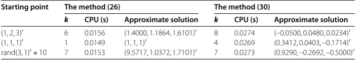
Table 1 Numerical results for Example 6.1

Starting point The method (26) The method (30)

k CPU (s) Approximate solution k CPU (s) Approximate solution

(1, 2, 3) 6 0.0156 (1.4000, 1.1864, 1.6101) 6 0.0262 (1.1798, 1.1380, 1.6447)

(1, 1, 1) 1 0.0149 (1, 1, 1) 1 0.0252 (1, 1, 1)

[image:10.595.113.480.575.635.2]

rand(3, 1)∗10 7 0.0153 (9.5717, 1.0372, 1.7101) 7 0.0270 (9.5717, 1.0372, 1.7101)

(1, 2, 3) 19 0.0166 (–0.3097, –0.1638, 0.1067) 5 0.0264 (–0.6409, –0.0027, 0.3205) (1, 1, 1) 5 0.0155 (0.3988, 0.0763, –0.2023) 10 0.0271 (0.1828, 0.0493, –0.1644) rand(3, 1)∗10 7 0.0159 (6.0095, –0.0363, –3.0054) 7 0.0280 (3.7284, 0.4046, –2.6730)

[image:10.595.117.479.671.732.2]

(11)

7 Conclusions

In this paper, by adopting the preconditioning techniques, a modiﬁed CQ algorithm is named preconditioning CQ algorithm, and its extensions for solving the ESFP have been presented. The approximate methods for how to estimate the preconditionerDare also discussed; the approximate diagonal preconditioner method does not need to compute the matrix inverses and the largest eigenvalue of the matrix AT_A_{. Thus, the algorithm} can be implemented easily. Moreover, the corresponding convergence property has been established in the feasible case of ESFP. The numerical results showed that the proposed algorithms and methods are eﬀective to solve some problems.

Competing interests

The authors declare that they have no competing interests.

Authors’ contributions

Both authors take equal roles in deriving results and writing of this paper. Both authors read and approved the ﬁnal manuscript.

Author details

1_{Department of Mathematics, Shijiazhuang Mechanical Engineering College, Shijiazhuang, 050003, China.}2_Department

of Mathematics and Information, Hebei Normal University, Shijiazhuang, 050016, China.

Acknowledgements

The authors would like to thank the associate editor and the referees for their comments and suggestions. This research was supported by the National Natural Science Foundation of China (11071053).

Received: 27 October 2013 Accepted: 3 April 2014 Published:06 May 2014

References

1. Censor, Y, Elfving, T: A multiprojection algorithm using Bregman projections in a product space. Numer. Algorithms8, 221-239 (1994)

2. Bauschke, HH, Borwein, JM: On projection algorithms for solving convex feasibility problems. SIAM Rev.38, 367-426 (1996)

3. Byrne, CL: A uniﬁed treatment of some iterative algorithms in signal processing and image reconstruction. Inverse Probl.20, 103-120 (2004)

4. Byrne, CL: Iterative projection onto convex sets using multiple Bregman distances. Inverse Probl.15, 1295-1313 (1999)

5. Byrne, CL: Bregman-Legendre multidistances projection algorithm for convex feasibility and optimization. In: Butnariu, D, Censor, Y, Reich, S (eds.) Inherently Parallel Algorithms in Feasibility and Optimization and Their Applications, pp. 87-100. Elsevier, Amsterdam (2001)

6. Byrne, CL: Iterative oblique projection onto convex sets and the split feasibility problem. Inverse Probl.18, 441-453 (2002)

7. Yang, QZ: The relaxed CQ algorithm solving the split feasibility problem. Inverse Probl.20, 1261-1266 (2004) 8. Qu, B, Xiu, N: A note on the CQ algorithm for the split feasibility problem. Inverse Probl.21, 1655-1665 (2005) 9. Wang, Z, Yang, Q: The relaxed inexact projection methods for the split feasibility problem. Appl. Math. Comput.217,

5347-5359 (2011)

10. Yang, Q, Zhao, J: The projection-type methods for solving the split feasibility problem. Math. Numer. Sin.28, 121-132 (2006) (in Chinese)

11. Xu, HK: Iterative methods for the split feasibility problem in inﬁnite-dimensional Hilbert spaces. Inverse Probl.26, 1-17 (2010)

12. López, G, Martín-Márquez, V, Wang, F, Xu, H-K: Solving the split feasibility problem without prior knowledge of matrix norms. Inverse Probl.28, 1-18 (2012)

13. Zarantonello, EH: Projections on convex sets in Hilbert space and spectral theory. In: Zarantonello, EH (ed.) Contributions to Nonlinear Functional Analysis. Academic Press, New York (1971)

14. Wang, F, Xu, HK: Approximating curve and strong convergence of the CQ algorithm for the split feasibility problem. J. Inequal. Appl.2010, Article ID 102085 (2010)

15. Abdellah, B, Muhammad, AN: On descent-projection method for solving the split feasibility problems. J. Glob. Optim.

54, 627-639 (2012)

16. Strand, ON: Theory and methods related to the singular-function expansion and Landweber’s iteration for integral equations of the ﬁrst kind. SIAM J. Numer. Anal.11, 798-825 (1974)

17. Piana, M, Bertero, M: Projected Landweber method and preconditioning. Inverse Probl.13, 441-463 (1997) 10.1186/1029-242X-2014-163