Volume 2009, Article ID 970723,16pages doi:10.1155/2009/970723
Research Article
Penalty Algorithm Based on Conjugate Gradient
Method for Solving Portfolio Management Problem
Zhong Wan,
1ShaoJun Zhang,
1and YaLin Wang
2 1School of Mathematics Sciences and Computing Technology, Central South University,Changsha, Hunan 410083, China
2School of Information Sciences and Engineering, Central South University, Changsha, Hunan 410083, China
Correspondence should be addressed to Zhong Wan,[email protected]
Received 17 December 2008; Revised 18 April 2009; Accepted 7 July 2009
Recommended by Kok Teo
A new approach was proposed to reformulate the biobjectives optimization model of portfolio management into an unconstrained minimization problem, where the objective function is a piecewise quadratic polynomial. We presented some properties of such an objective function. Then, a class of penalty algorithms based on the well-known conjugate gradient methods was developed to find the solution of portfolio management problem. By implementing the proposed algorithm to solve the real problems from the stock market in China, it was shown that this algorithm is promising.
Copyrightq2009 Zhong Wan et al. This is an open access article distributed under the Creative Commons Attribution License, which permits unrestricted use, distribution, and reproduction in any medium, provided the original work is properly cited.
1. Introduction
Portfolio management problem concerns itself with allocating one’s assets among alternative securities to maximize the return of assets and to minimize the investment risk. The pioneer work on this problem was Markowitz’s mean variance model1, and the solution of his mean-variance methodology has been the center of the consequent research activities and forms the basis for the development of modern portfolio management theory. Commonly, the portfolio management problem has the following mathematical description.
Assume that there are n kinds of securities. The return rate of the jth security is denoted asRj,j1, . . . , n. Letxjbe the proportion of total assets devoted to thejth security, then it is obvious that
n
j1
In the real setting, due to uncertainty, the return ratesRj,j 1,2, . . . n, are random parameters. Hence, the total return of the assets
Rx n j1
Rjxj 1.2
is also random. In this situation, the risk of investment has to be taken into consideration. In the classical model, this risk is measured by the variance ofRx. IfV ∈Rn×nis the covariance matrix of the vectorR R1, R2, . . . , RnT, then the variance ofRxis
VRx xTV x. 1.3
Therefore, a portfolio management problem can be formulated into the following biobjectives programming problem:
maximize Rx RTx,
minimize VRx xTV x,
subject to eTx1,
1≥x≥0,
1.4
wheree is a vector of all ones. Up to our knowledge, almost all of the existing models of portfolio management problems evolved from the basic model1.4.
Summarily, the past attempts on the portfolio management problems concentrated on two major issues. The first one is to propose new models. In this connection, some recent notable contributions mainly include the following:
imean-absolute deviation modelSimaan2,
iimaximizing probability modelWilliams3,
iiidifferent types of mean-variance modelsBest and Jaroslava4, Konna and Suzuki
5and Yoshimoto6,
ivmin-max modelsCai et al.7, Deng et al.8,
vinterval programming modelsGiove et al.9, Ida10, Lai et al.11,
vifuzzy goal programming modelParra et al.12,
viiadmissible efficient portfolio selection modelZhang and Nie13,
ixupper and lower exponential possibility distribution based modelTanaka and Guo
15,
xmodel with fuzzy probabilitiesHuang16,17, Tanaka and Guo15.
The second issue is about the numerical solution algorithms for the distinct models. One of the fundamental ways is to reformulate 1.4 into a deterministic single-objective optimization problem. For example, in the researches of Best4,18, Pang 19, Kawadai and Konno20, Perold21, Sharpe22, Szeg ¨o23and Yoshimoto6, they assumed that the return of each security, the variance, and the covariances among them can be estimated by the investor prior to decision. Under this assumption, the problem1.4is a deterministic problem. Furthermore, if an aversion coefficientλ is introduced, the problem 1.4 can be transformed into the following standard quadratic programming problem:
minimize fx −1−λμTx λxTV x
subject to eTx1,
b≥x≥a,
1.5
whereμ∈Rnis the expected value vector ofR, anda, b∈Rnare two given vectors denoting the lower and the upper bounds of decision vector, respectively.
Obviously, ifλ 0 in1.5, then it implies that the return is maximized regardless of the investment risk. On the other hand, if λ 1, then the risk is minimized without consideration on the investment income. Increasing value ofλin the interval0,1indicates an increasingly weight of the invest risk, and vice versa.
For a fixed λ ∈ 0,1, it is noted that 1.5 is a quadratic programming problem. Since it has been shown that the matrix V is positive semidefinite, the problem1.5 is a convex quadratic programming CQP. For a CQP, there exist a lot of efficient methods to find its minimizers. Among them, active-set methods, interior-point methods, and gradient-projection methods have been widely used since the 1970s. For their detailed numerical performances, one can see 24–30 and the references therein. However, the efficiency of those methods seriously depends on the factorization techniques of matrix at each iteration, often exploiting the sparsity in V for a large-scale quadratic programming. So, from the viewpoint of smaller storage requirements and computation cost, the methods mentioned above must not be most suitable for solving the problem 1.5 if V is a dense matrix.
Fortunately, recent research shows that the conjugate gradient methods can remedy the drawback in factorization of Hessian matrix for an unconstrained minimization problem. At each conjugate-gradient iteration, it is only involved with computing the gradient of objective function. For details in this direction, see, for example,31–34.
The lay out of the paper is as follows.Section 2is devoted to the reformulation of the original constrained problem. Some features of the subproblem will be presented. Then, in
Section 3, we are going to develop a penalty algorithm based on conjugate gradient methods.
Section 4will provide applications of the proposed algorithm. The last section concludes with some final remarks.
2. Reformulation
Firstly, for brevity, denote
ccj
n×1−1−λμ, Q
qij
n×n2λV. 2.1
Then, the problem1.5reads
minimize fx cTx 1
2x TQx
subject to eTx1,
a≤x≤b.
2.2
Since the covariance matrix V is symmetric positive semidefinite, Q also has such property. Thus,fxis a convex function.
For the equality constrainteTx1 and the inequality constraintsa≤x≤bin2.2, we define a functionP :Rn 1 → R, which is used to describe the constraints violation:
Px;θ θ 2
eTx−12 minx−a,02 minb−x,02
, 2.3
whereθ >0 is called penalty parameter, and·denotes the 2-norm of vector. Ifxis a feasible point of problem2.2, then
Px;θ 0. 2.4
Actually, the larger the absolute value ofPx;θis, the furtherxfrom the feasible region is. The functionF:Rn 1 → R,
Fx;θ cTx 1
2x TQx
θ
2
eTx−12 minx−a,02 minb−x,02
2.5
features:
1Fis a piecewise quadratic polynomial;
2Fis piecewise continuously differentiable;
3IfQis positive semidefinite, thenFis a piecewise convex quadratic function.
For example, letn2, and denote
cx;θ ⎧ ⎪ ⎪ ⎪ ⎪ ⎪ ⎪ ⎪ ⎪ ⎪ ⎪ ⎪ ⎪ ⎪ ⎪ ⎪ ⎪ ⎪ ⎪ ⎪ ⎪ ⎪ ⎪ ⎪ ⎪ ⎪ ⎪ ⎪ ⎪ ⎪ ⎪ ⎪ ⎪ ⎪ ⎪ ⎪ ⎪ ⎪ ⎪ ⎪ ⎪ ⎪ ⎪ ⎪ ⎪ ⎪ ⎪ ⎪ ⎪ ⎪ ⎪ ⎪ ⎪ ⎪ ⎪ ⎪ ⎪ ⎪ ⎪ ⎪ ⎪ ⎪ ⎪ ⎪ ⎪ ⎪ ⎪ ⎪ ⎪ ⎪ ⎪ ⎪ ⎪ ⎪ ⎪ ⎪ ⎪ ⎪ ⎪ ⎪ ⎪ ⎨ ⎪ ⎪ ⎪ ⎪ ⎪ ⎪ ⎪ ⎪ ⎪ ⎪ ⎪ ⎪ ⎪ ⎪ ⎪ ⎪ ⎪ ⎪ ⎪ ⎪ ⎪ ⎪ ⎪ ⎪ ⎪ ⎪ ⎪ ⎪ ⎪ ⎪ ⎪ ⎪ ⎪ ⎪ ⎪ ⎪ ⎪ ⎪ ⎪ ⎪ ⎪ ⎪ ⎪ ⎪ ⎪ ⎪ ⎪ ⎪ ⎪ ⎪ ⎪ ⎪ ⎪ ⎪ ⎪ ⎪ ⎪ ⎪ ⎪ ⎪ ⎪ ⎪ ⎪ ⎪ ⎪ ⎪ ⎪ ⎪ ⎪ ⎪ ⎪ ⎪ ⎪ ⎪ ⎪ ⎪ ⎪ ⎪ ⎪ ⎪ ⎩ ⎛ ⎝c1−θ
c2−θ ⎞
⎠, x∈D1 x1, x2T :
a1≤x1≤b1, a2≤x2≤b2
,
⎛
⎝c1−θ−θa1
c2−θ ⎞
⎠, x∈D2 x1, x2T :
x1< a1, a2≤x2≤b2
,
⎛
⎝c1−θ−θb1
c2−θ ⎞
⎠, x∈D3 x1, x2T :x
1> b1, a2≤x2 ≤b2
,
⎛
⎝ c1−θ
c2−θ−θa2 ⎞
⎠, x∈D4 x1, x2T :a
1≤x1≤b1, x2 < a2
,
⎛
⎝ c1−θ
c2−θ−θb2 ⎞
⎠, x∈D5 x1, x2T :a
1≤x1≤b1, x2 > b2
,
⎛
⎝c1−θ−θa1
c2−θ−θa2 ⎞
⎠, x∈D6 x1, x2T :
x1< a1, x2 < a2
,
⎛
⎝c1−θ−θa1
c2−θ−θb2 ⎞
⎠, x∈D7 x1, x2T :
x1< a1, x2 > b2
,
⎛
⎝c1−θ−θb1
c2−θ−θa2 ⎞
⎠, x∈D8 x1, x2T :x
1> b1, x2< a2
,
⎛
⎝c1−θ−θb1
c2−θ−θb2 ⎞
⎠, x∈D9 x1, x2T :x
1> b1, x2> b2
Qx;θ ⎧ ⎪ ⎪ ⎪ ⎪ ⎪ ⎪ ⎪ ⎪ ⎪ ⎪ ⎪ ⎪ ⎪ ⎪ ⎪ ⎪ ⎪ ⎪ ⎪ ⎪ ⎪ ⎪ ⎨ ⎪ ⎪ ⎪ ⎪ ⎪ ⎪ ⎪ ⎪ ⎪ ⎪ ⎪ ⎪ ⎪ ⎪ ⎪ ⎪ ⎪ ⎪ ⎪ ⎪ ⎪ ⎪ ⎩ ⎛
⎝q11 θ q12 θ
q21 θ q22 θ ⎞
⎠, x∈D1,
⎛
⎝q11 2θ q12 θ
q21 θ q22 θ ⎞
⎠, x∈D2∪D3,
⎛
⎝q11 θ q12 θ
q21 θ q22 2θ ⎞
⎠, x∈D4∪D5,
⎛
⎝q11 2θ q12 θ
q21 θ q22 2θ ⎞
⎠, x∈D6∪D7∪D8∪D9.
2.6
Then,Fx;θhas the following more compact form:
Fx;θ c0 cx;θTx 1 2x
TQx;θx, 2.7
wherec0is a constant scalar.
Next, we are going to present some properties ofF.
Proposition 2.1. Givenn, the piecewise functionFconsists of
20C0n 2C1n 22Cn2 · · · 2nCnn 2.8
pieces.
Proposition 2.2. Assume thatk≤n. For any{i1, i2, . . . , ik } ⊆ {1,2. . . , n}, define a matrix
Ai1i2···ik
⎛ ⎜ ⎜ ⎜ ⎜ ⎜ ⎜ ⎜ ⎜ ⎜ ⎜ ⎜ ⎜ ⎜ ⎜ ⎜ ⎜ ⎜ ⎜ ⎜ ⎜ ⎜ ⎜ ⎜ ⎝ . ..
1 2 1 1 1 1 1 1
. ..
1 1 1 2 1 1 1 1
. .. . ..
1 1 1 1 1 1 2 1
. .. ⎞ ⎟ ⎟ ⎟ ⎟ ⎟ ⎟ ⎟ ⎟ ⎟ ⎟ ⎟ ⎟ ⎟ ⎟ ⎟ ⎟ ⎟ ⎟ ⎟ ⎟ ⎟ ⎟ ⎟ ⎠ .. . · · · · · · ·i1
.. .
· · · ·i2
.. . .. .
· · · ·ik
.. .
, 2.9
1RAi1i2···ik k 1, whereR·denotes the rank of a matrix.
2For a fixed k, all matrices Ai1i2···ik, where{i1, i2, . . . , ik} ⊆ {1,2, . . . , n}, have the same
eigenvalues and eigenvectors.
3Whenk < n−1, all matricesAi1i2···ik, where{i1, i2, . . . , ik} ⊆ {1,2, . . . , n}, have nonnegative
eigenvalue, and hence they are positive semidefinite. When k ≥ n−1, they are positive definite matrices.
Proof. From the construction ofFand the linear algebra theory, it is not difficult to prove the above two propositions. We omit it.
In the following, we turn to state the relation between the global minimizer ofFand that of the original problem1.5.
Theorem 2.3. For a given sequence{θk}, suppose thatθk → ∞ask → ∞. Letxkbe an exact
global minimizer ofFx;θk. Then, every accumulation pointx∗of{xk}is a solution of problem
1.5.
Proof. Letxbe a global solution of problem1.5. Then, for any feasible pointx, we have
fx≤fx. 2.10
Sincexkis an exact global minimizer ofFx;θkfor the fixedθk, it follows that
Fxk;θk≤Fx;θk. 2.11
By definition,2.11is equivalent to
fxk θk
2
eTxk−12 minxk−a,02 minb−xk,02
≤fx θk
2
eTx−12 minx−a,02 minb−x,02
fx,
2.12
where the last equality is from the feasibility ofx. So, it is obtained that
eTxk−12 minxk−a,02 minb−xk,02≤ 2 θk
fx−fxk. 2.13
Letx∗be an accumulation point of{xk}. Without loss of generality, assume that
lim k→ ∞x
Then, by taking the limit ofk → ∞on both sides of2.13, we have
0≤eTx∗−12 minx∗−a,02 minb−x∗,02
≤ lim k→ ∞
2
θk
fx−fxk0,
2.15
where the last equality follows fromθk → ∞. It follows that
eTx∗1, a≤x∗≤b. 2.16
Therefore, we have proved thatx∗is a feasible point.
In the following, we prove thatx∗is a global minimizer of problem1.5. Because
fx∗≤fx∗ lim k→ ∞
θk
2
eTxk−12 minxk−a,02 minb−xk,02
≤fx,
2.17
x∗is a global minimizer off.
The desired result has been proved.
Without difficulty, the following result can be proved.
Theorem 2.4. Suppose thatxis a solution of problem1.5. Then,xis a global minimizer ofF·;θ
for anyθ.
Based on Theorems2.3and2.4, we will develop an algorithm to search for a solution of problem1.5by solving a sequence of piecewise quadratical programming problems.
3. Penalty Algorithm Based on Conjugate Gradient Method
Among all methods for the unconstrained optimization problems, the conjugate gradient method is regarded as one of the most powerful approaches due to its smaller storage requirements and computation cost. Its priorities over other methods have been addressed in many literatures. For example, in27,32,34–38, the global convergence theory and the detailed numerical performances on the conjugate gradient methods have been extensively investigated.
Regarding the coefficients of the quadratic terms in
θ
2
minx−a,02 minb−x,02, 3.1
we modifyQ qijaccording to the following update rule:
qij
⎧ ⎪ ⎪ ⎪ ⎨ ⎪ ⎪ ⎪ ⎩
qij, ifi /j,
qii, ifij, ai≤xi≤bi,
qii θ
, ifij, ai> xi orxi> bi.
3.2
Regarding the coefficients of the linear terms in
θ
2
minx−a,02 minb−x,02, 3.3
we modifyc ciaccording to the following update rule:
ci
⎧ ⎪ ⎪ ⎪ ⎨ ⎪ ⎪ ⎪ ⎩
ci, ifai≤xi≤bi,
ci−θai, ifxi< ai, ci−θbi, ifxi> bi.
3.4
Define
QQ θeeT, cc−θe. 3.5
The conjugate gradient method will be employed into an ordinary minimization of quadratic function:
minFx;θ c0 cTx 1 2x
TQx, 3.6
whereθis a given parameter. It is easy to see that
∇Fxx;θ Qx c. 3.7
1At the current iterate pointxl, determinate a search direction:
dl
⎧ ⎨ ⎩
−Qx0 c forl0, −Qxl c βldl−1 forl≥1,
3.8
whereβlis chosen such thatdlis a conjugate direction ofdl−1with respect to the matrixQ.
2Along the directiondl, choose a step sizeαlsuch that, at the new iterate point
xl 1xl α
ldl, 3.9
the absolute value of the functionF·;θdecreases sufficiently.
The following lemma presents a method to determine the search direction.
Lemma 3.1. If
βl
Qxl cTQdl−1
dl−1T
Qdl−1 ,
3.10
dl−Qxl c βldl−1, 3.11
thendlin3.8is a conjugate direction ofdl−1with respect toQ.
Proof. Owing to
dlTQdl−1−Qxl c βldl−1
T Qdl−1
−Qxl c Qxl cTQdl−1 dl−1TQdl−1 d
l−1
T Qdl−1
0,
3.12
the desired result is obtained.
Actually, the formula3.10is called HS method.
In the case that the step sizeαlis chosen by exact linear search along the directiondl, that is,
αl−
Qxl cTdl
dlTQdl ,
3.13
Theorem 3.2. Letx0be an arbitrary initial vector. Let{xl, l1,2, . . .}be a sequence generated by
the conjugate gradient algorithm defined by3.8–3.13. Then, either
lim l→ ∞F
xl;θ−∞, 3.14
or
lim inf∇xFxl;θ0. 3.15
In particular, ifx∗is an accumulation point of the sequence{xl :l 1,2, . . .}, thenx∗is a global minimizer ofF·;θ.
Remark 3.3. Ifβlis computed by
βl
Qxl c2
Qxl−1 c2
, 3.16
then the results inTheorem 3.2still hold. Equation3.16is called FR method.
Based on the discussion above, we now come to develop a penalty algorithm based on conjugate gradient method in the last of this section.
Algorithm 1Penalty Algorithm Based on Conjugate Gradient Method.
Step 0Initialization. Given constant scalarsθ >1,λ ∈0,1,δ > 0,ε > 0 andρ. Input the expected return vectorμ, and computeQandc. Choose an initial solution x0. Setk : 0, l:0, andxl:xk.
Step 1Reformulation. If
Qxl c≤ε, 3.17
then set
xk:xl, 3.18
and go toStep 4; otherwise, go toStep 2.
Step 2Search Direction. Compute the search directiondlby3.8and3.10.
Step 3Exact Line Search. Computeαlby3.13, and update
xl:xl αldl
. 3.19
Table 1:Numerical performance ofAlgorithm 1.
Problem n CPU of HS CPU of FR k θ Px∗;θ∗
1 10 1 1 3 104 2.5652e−005
2 20 1 8 3 104 1.3314e−005
3 30 1 5 3 104 5.9817e−005
4 40 4 58 4 105 1.1302e−005
5 50 2 11 4 105 2.4787e−005
6 60 2 46 3 104 8.5817e−005
7 70 4 12 4 105 1.7759e−005
8 80 4 143 4 105 2.8436e−005
9 90 2 126 4 105 9.6836e−005
10 100 3 648 4 105 4.8977e−005
Step 4Feasibility Test. Check feasibility ofxkin problem2.2. If
Pxk;θ≤δ, 3.20
the algorithm terminates; otherwise, go toStep 5.
Step 5Update. Setl:0,xl:xk,θ:ρθ. At the new iterate pointxk, modify the matrix
Qand the vectorcby3.2and3.4, respectively. Setk:k 1, and return toStep 1.
Remark 3.4. 1In Algorithm 1, the index k denotes the number of updating penalty parameter, and l denotes the number of iterations of conjugate gradient method for unconstrained subproblem3.6.
2For some fixedθ, it is easy to see that the condition
Pxk;θ θ k
2
eTxk−12 minxk−a,02 minb−xk,02
≤δ 3.21
implies thatxkis feasible. FromTheorem 2.3, it leads thatxkis a global minimizer of the original problem1.5ifxkis a global minimizer of problem3.6.
4. Numerical Experiments
In this section, we are going to test the effectiveness ofAlgorithm 1. All the test problems come from the real stock market in China, in 2007. The computer procedures are implemented on MATLAB 6.5.
In our numerical experiments, the initial solution is chosen to satisfy
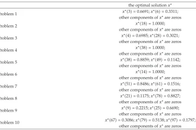
Table 2:Optimal solutions of the ten problems.
the optimal solutionx∗
Problem 1 x∗3 0.6691;x∗6 0.3311;
other components ofx∗are zeros
Problem 2 x∗18 1.0000;
other components ofx∗are zeros
Problem 3 x∗4 0.6985;x∗28 0.3021;
other components ofx∗are zeros
Problem 4 x∗38 1.0000;
other components ofx∗are zeros
Problem 5 x∗38 0.8859;x∗49 0.1142;
other components ofx∗are zeros
Problem 6 x∗14 1.0000;
other components ofx∗are zeros
Problem 7 x∗51 0.8486;x∗61 0.1516;
other components ofx∗are zeros
Problem 8 x∗21 0.1175;x∗78 0.8827;
other components ofx∗are zeros
Problem 9 x∗9 0.2215;x∗25 0.6690;
other components ofx∗are zeros
Problem 10 x∗67 0.3086;x∗79 0.5138;x∗97 0.1797;
other components ofx∗are zeros
the bound vectorais a vector of all zeros, andbis a vector of all ones. We take the initial penalty parameterθ10 and the aversion coefficientλ0.5. The tolerance of error is taken as
ε10−7, δ10−4. 4.2
We implementAlgorithm 1to solve ten real problems. Each of them has a different dimension ranging from 10 to 100. In these problems, the expected return rates of each stock come from the monthly data in the stock market of China, in 2007. InTable 3, we list the data used to form a real problem whose size of dimension is 30.
InTable 1, we report the numerical behavior ofAlgorithm 1for all ten problems. InTable 1,nis the dimensional size of each problem; the third and the forth columns report the CPU time when βl is evaluated by HS method and FR method, respectively.k indicates the number of updating penalty parameter,θis the penalty parameter, andPx∗;θ∗
denotes the value of penalty term.
InTable 2, we list the obtained optimal solution for each problem.
5. Final Remarks
Table 3:The return rates collected from the stock market in China, 2007.
1 2 3 4 5 6 7 8 9 10 11 12
No.1 0.4600 0.1900 0.1800 0.1130 0.2400 0.4600 0.4200 0.1500 0.1700 0.1140 0.2100 0.4200 No.2 0.6420 0.6560 0.6630 0.6990 0.6080 0.5420 0.6210 0.5550 0.6590 0.5810 0.6850 0.6210 No.3 0.1190 0.0590 0.2100 0.1100 0.1200 0.1190 0.1280 0.0580 0.2100 0.1100 0.1300 0.1280 No.4 0.0800 −0.0350 −0.2540 0.0830 0.0960 0.0800 0.1000 −0.0340 −0.2440 0.1100 0.1200 0.1000 No.5 0.7170 0.0940 0.4400 0.1430 0.6880 0.7170 0.7080 0.0190 0.3100 0.1470 0.6810 0.7080 No.6 0.0151 0.0105 0.0749 0.0081 0.0133 0.0151 0.0179 0.0083 0.0309 0.0090 0.1390 0.0179 No.7 0.2530 0.2430 0.3100 0.0480 0.1500 0.2530 0.2470 0.2440 0.3000 0.0480 0.1500 0.2470 No.8 0.3400 0.3006 0.3500 0.2280 0.4800 0.3400 0.3400 0.3026 0.3500 0.2270 0.4800 0.3400 No.9 0.0804 0.0579 0.1190 0.0420 0.0600 0.0804 0.0833 0.0597 0.1070 0.0430 0.0600 0.0833 No.10 0.0360 0.0230 0.0300 0.0140 0.0360 0.0360 0.0740 0.0210 0.0420 0.0150 0.0540 0.0740 No.11 0.0050 0.0130 0.0234 0.0020 0.0020 0.0050 0.0046 0.0130 0.0187 0.0020 0.0014 0.0046 No.12 0.2897 0.3100 0.4303 0.1153 0.1930 0.2897 0.2893 0.3200 0.3893 0.1151 0.1927 0.2893 No.13 0.7690 0.8060 0.9050 0.5340 0.4980 0.7690 0.7670 0.8090 0.8600 0.4350 0.5700 0.7670 No.14 0.0160 0.0110 0.0258 0.0006 0.0050 0.0160 −0.0230 0.0170 0.0171 −0.0242 −0.0220−0.0230 No.15 0.0820 0.0370 0.0640 0.0200 0.0550 0.0820 0.0770 0.0370 0.0690 0.0200 0.0490 0.0770 No.16 0.4714 0.3607 0.6000 0.1275 0.2700 0.4714 0.4295 0.3585 0.5700 0.1275 0.2600 0.4295 No.17 0.2280 0.0950 0.1240 0.0820 0.1650 0.2280 0.2150 0.0970 0.1250 0.0812 0.1520 0.2150 No.18 0.0107 0.0053 0.0120 0.0040 0.0070 0.0107 0.0108 0.0416 −0.0400 0.0040 0.0120 0.0108 No.19 0.1400 0.2000 0.2400 0.0518 0.1100 0.1400 0.1400 0.2000 0.2300 0.0512 0.1200 0.1400 No.20 0.1500 0.1600 0.2100 0.0400 0.1100 0.1500 0.1500 0.1500 0.2000 0.0400 0.1100 0.1500 No.21 0.9850 1.3137 1.3200 0.2567 0.6100 0.9850 0.8130 1.3179 1.2900 0.1336 0.4300 0.8130 No.22 0.4717 0.4800 0.5730 0.0150 0.4271 0.4717 0.4285 0.2500 0.2338 0.0130 0.3816 0.4285 No.23 0.2500 0.1250 0.3300 0.0780 0.2000 0.2500 0.2400 0.1260 0.3400 0.0770 0.2000 0.2400 No.24 0.0310 0.0600 0.0880 0.0060 0.0300 0.0310 0.0240 0.0600 0.0950 0.0060 0.0190 0.0240 No.25 0.1190 0.0590 0.2100 0.1100 0.1200 0.1190 0.1280 0.0580 0.2100 0.1100 0.1300 0.1280 No.26 0.0110 0.0139 0.0140 0.0040 0.0090 0.0110 0.0020 0.0137 0.0080 0.0010 0.0010 0.0020 No.27 0.0100 0.0640 0.0515 −0.0350 0.0040 0.0100 −0.0700 0.0630 −0.0061 −0.0690 −0.0733−0.0700 No.28 0.2680 0.2770 0.4320 0.0230 0.1900 0.2680 0.2680 0.2740 0.4320 0.0220 0.1880 0.2680 No.29 0.0061 −0.0060 −0.6742 0.0033 0.0050 0.0061 0.0131 −0.0220 −0.4474 0.0039 0.0099 0.0131 No.30 0.0600 −0.2200 −2.2300 0.0250 0.0400 0.0600 0.0450 −0.0100 −1.5700 0.0080 0.0300 0.0450
Regarding the features of the optimization models in portfolio management, a class of penalty algorithms based on the conjugate gradient method was developed. The numerical performance of the proposed algorithm in solving the real problems verifies its effectiveness.
Acknowledgments
References
1 H. Markowitz, “Portfolio selection,”Journal of Finance, vol. 7, pp. 77–91, 1952.
2 Y. Simaan, “Estimation risk in portfolio selection: the mean variance model versus the mean absolute deviation model,”Management Science, vol. 43, pp. 1437–1446, 1997.
3 J. O. Williams, “Maximizing the probability of achieving investment goals,” Journal of Portfolio Management, vol. 24, pp. 77–81, 1997.
4 M. J. Best and H. Jaroslava, “The efficient frontier for bounded assets,” Mathematical Methods of Operations Research, vol. 52, no. 2, pp. 195–212, 2000.
5 H. Konno and K. Suzuki, “A mean-variance-skewness optimization model,”Journal of Operations Research Society of Japan, vol. 38, pp. 137–187, 1995.
6 A. Yoshimoto, “The mean-variance approach to portfolio optimization subject to transaction costs,”
Journal of the Operations Research Society of Japan, vol. 39, no. 1, pp. 99–117, 1996.
7 X. Cai, K. L. Teo, X. Yang, and X. Y. Zhou, “Portfolio optimization under a minimax rule,”Management Science, vol. 46, no. 7, pp. 957–972, 2000.
8 X. T. Deng, Z. F. Li, and S. Y. Wang, “A minimax portfolio selection strategy with equilibrium,”
European Journal of Operational Research, vol. 166, no. 1, pp. 278–292, 2005.
9 S. Giove, S. Funari, and C. Nardelli, “An interval portfolio selection problem based on regret function,”European Journal of Operational Research, vol. 170, no. 1, pp. 253–264, 2006.
10 M. Ida, “Solutions for the portfolio selection problem with interval and fuzzy coefficients,”Reliable Computing, vol. 10, no. 5, pp. 389–400, 2004.
11 K. K. Lai, S. Y. Wang, J. P. Xu, S. S. Zhu, and Y. Fang, “A class of linear interval programming problems and its application to portfolio selection,”IEEE Transactions on Fuzzy Systems, vol. 10, no. 6, pp. 698– 704, 2002.
12 M. A. Parra, A. B. Terol, and M. V. R. Uria, “A fuzzy goal programming approach to portfolio selection,”European Journal of Operational Research, vol. 133, no. 2, pp. 287–297, 2001.
13 W. G. Zhang and Z. K. Nie, “On admissible efficient portfolio selection problem,”Applied Mathematics and Computation, vol. 159, pp. 357–371, 2004.
14 C. Carlsson, R. Full´er, and P. Majlender, “A possibilistic approach to selecting portfolios with highest utility score,”Fuzzy Sets and Systems, vol. 131, no. 1, pp. 13–21, 2002.
15 H. Tanaka and P. Guo, “Portfolio selection based on upper and lower exponential possibility distributions,”European Journal of Operational Research, vol. 114, pp. 115–126, 1999.
16 X. X. Huang, “Fuzzy chance-constrained portfolio selection,”Applied Mathematics and Computation, vol. 177, no. 2, pp. 500–507, 2006.
17 X. X. Huang, “Two new models for portfolio selection with stochastic returns taking fuzzy information,”European Journal of Operational Research, vol. 180, no. 1, pp. 396–405, 2007.
18 M. J. Best and R. R. Grauer, “The efficient set mathematics when mean-variance problems are subject to general linear constrains,”Journal of Economics and Business, vol. 42, pp. 105–120, 1990.
19 J. S. Pang, “A new and efficient algorithm for a class of portfolio selection problems,”Operations Research, vol. 28, no. 3, part 2, pp. 754–767, 1980.
20 N. Kawadai and H. Konno, “Solving large scale mean-variance models with dense non-factorable covariance matrices,”Journal of the Operations Research Society of Japan, vol. 44, no. 3, pp. 251–260, 2001.
21 A. F. Perold, “Large-scale portfolio optimization,”Management Science, vol. 30, no. 10, pp. 1143–1160, 1984.
22 W. F. Sharpe,Portfolio Theory and Capital Markets, McGraw-Hil, New York, NY, USA, 1970.
23 G. P. Szeg ¨o,Portfolio Theory, Economic Theory, Econometrics, and Mathematical Economics, Academic Press, New York, NY, USA, 1980.
24 E. D. Andersen, J. Gondzio, C. Meszaros, and X. Xu, “Implementation of interior-point methods for large scale linear programs,” inInterior Point Methods of Mathematical Programming, vol. 5 ofApplied Optimization, pp. 189–252, Kluwer Academic Publishers, Dordrecht, The Netherlands, 1996.
25 J. Gondzio and A. Grothey, “Parallel interior-point solver for structured quadratic programs: application to financial planning problems,”Annals of Operations Research, vol. 152, pp. 319–339, 2007. 26 S. Mehrotra, “On the implementation of a primal-dual interior point method,”SIAM Journal on
27 J. Nocedal and S. J. Wright,Numerical Optimization, Springer Series in Operations Research and Financial Engineering, Springer, New York, NY, USA, 2nd edition, 2006.
28 F. Potra, C. Roos, and T. Terlaky, Eds.,Special Issue on Interior-Point Methods, Optimization Method and Software, vol. 11-12, 1999.
29 M. V. Solodov and P. Tseng, “Modified projection-type methods for monotone variational inequalities,”SIAM Journal on Control and Optimization, vol. 34, no. 5, pp. 1814–1830, 1996.
30 T. F. Coleman and L. A. Hulbert, “A direct active set algorithm for large sparse quadratic programs with simple bounds,”Mathematical Programming, vol. 45, no. 3, pp. 373–406, 1989.
31 N. Andrei, “A Dai-Yuan conjugate gradient algorithm with sufficient descent and conjugacy conditions for unconstrained optimization,”Applied Mathematics Letters, vol. 21, no. 2, pp. 165–171, 2008.
32 Y. Dai and Q. Ni, “Testing different conjugate gradient methods for large-scale unconstrained optimization,”Journal of Computational Mathematics, vol. 21, no. 3, pp. 311–320, 2003.
33 Z.-J. Shi and J. Shen, “Convergence of Liu-Storey conjugate gradient method,” European Journal of Operational Research, vol. 182, no. 2, pp. 552–560, 2007.
34 J. Sun, X. Yang, and X. Chen, “Quadratic cost flow and the conjugate gradient method,”European Journal of Operational Research, vol. 164, no. 1, pp. 104–114, 2005.
35 Y. H. Dai and Y. Yuan, “Convergence properties of the conjugate descent method,” Advances in Mathematics, vol. 25, no. 6, pp. 552–562, 1996.
36 Y. Liu and C. Storey, “Efficient generalized conjugate gradient algorithms. I. Theory,” Journal of Optimization Theory and Applications, vol. 69, no. 1, pp. 129–137, 1991.
37 J. Nocedal, “Conjugate gradient methods and nonlinear optimization,” in Linear and Nonlinear Conjugate Gradient-Related Methods, L. Adams and J. L. Nazareth, Eds., pp. 9–23, SIAM, Philadelphia, Pa, USA, 1996.