Agricultural production in the state of rio grande do sul / Brazil: An analysis from the estimation of the cobb douglas production function

Full Length Research Article

AGRICULTURAL PRODUCTION IN THE STATE OF RIO GRANDE DO SUL / BRAZIL: AN ANALYSIS

FROM THE ESTIMATION OF THE COBB DOUGLAS PRODUCTION FUNCTION

*1

_{Nilson Luiz Costa,}

_{Antônio Cordeiro De Santana,}

_{Carlos André Corrêa De Mattos and}

4

_{Antônio Joreci Flores}

1

_{Av. Independência, nº 3751. Bairro Vista Alegre. Palmeira das Missões, RS – Brazil, CEP: 98300-000, Brazil}

_{Av. Tancredo Neves, 2501. Montese. 66077530 - Belém, PA – Brazil}

3

_{ICSA - Campus Universitário do Guamá, Rua Augusto Corrêa, N º 1 – UFPA. 66075-110- Belém, PA – Brazil}

_{Av. Independência, nº 3751, Bairro Vista Alegre. 98300-000 - Palmeira das Missões / RS / Brazil}

ARTICLE INFO ABSTRACT

Agribusiness plays a very significant role in the economy of the Brazilian state of Rio Grande do Sul because it generates jobs and income in rural and urban areas. The aim of this study was to evaluate the relationship between factors of production and gross output value in farms. Such analysis can underpin policies for maximization of the economic result of agricultural output. Thus, data from the Brazilian Agricultural Census (2006) were used for an estimation of the Cobb-Douglas production function. Among the findings, it is noteworthy that the existing capital within the rural establishments is the variable that accounts for most of the Gross Output Value of Agricultural Production. It was also observed that the returns to scale are decreasing and that the average productivity of factors is not homogeneous across microregions. As a result, this paper underlined the need for further research and public policies that can contribute to the modernization and increased agricultural productivity.

Copyright © 2015 Nilson Luiz Costa et al.This is an open access article distributed under the Creative Commons Attribution License, which permits unrestricted use, distribution, and reproduction in any medium, provided the original work is properly cited.

INTRODUCTION

The economy of the state of Rio Grande do Sul, as compared to the economic activity of other Brazilian states, stands out for production in three sectors: primary, secondary and tertiary. Productive activities ensure much of the domestic market supply and make it one of the largest Brazilian exporters. With a Gross Domestic Product (GDP) estimated at BRL 215.86 billion in 2009, Rio Grande do Sul ranked fourth among the highest GDPs in Brazil. The GDP per capita, equivalent to BRL 19,778.39, is greater than the average GDP per capita of Brazil, BRL 16,917.66 (Brasil, 2011). In the 496 towns and cities in the state, 441,467 farms, predominantly small and mid-sized ones, produce food and fiber in an area of approximately 18.9 million hectares and generate employment for 1.07 million rural workers (Brasil, 2009). Investments on the technology used in the production processes of rural establishments were estimated from the cost spent on modern

*Corresponding author: Nilson Luiz Costa

Av. Independência, nº 3751. Bairro Vista Alegre. Palmeira das Missões, RS – Brazil, CEP: 98300-000, Brazil

inputs: BRL 1.93 billion on fertilizers, BRL 1.26 billion on soil amendments, BRL 268.27 million on seeds and seedlings, BRL 1.11 billion on pesticides and BRL 893.54 million on salt and feeds, among others (Brasil, 2009). The structure of production and marketing is comprised of 166 agricultural cooperatives joined by approximately 272,882 associates (2010), with sales of BRL 14.94 billion and 30,275 formal jobs (Ocergs, 2012). Agriculture, forestry and silviculture correspond to 68.7% of gross value added of agriculture, while livestock and fisheries account for 31.3%. The economic output of the agricultural sector in Rio Grande do Sul represents 9.9% of total amount in the state, while industrial activity accounts for 29.2% and services, 60.9% (Brazil, 2011). The importance of agricultural production for socioeconomics in the state of Rio Grande do Sul justifies the formulation of public policies to stimulate this sector, but the planning of agricultural policy necessarily depends on solid knowledge of the structure and situation of the productive sector. In this context, the study of factors that influence production can be another tool for planning policies for agribusiness in Rio Grande do Sul. Aligned with these principles, this paper is aimed at estimating the function of

ISSN: 2230-9926

International Journal of Development Research

Vol. 5, Issue, 07, pp. 4916-4922, July, 2015

DEVELOPMENT RESEARCH

Article History: Received 30th _{April, 2015}

Received in revised form 14th _{May, 2015}

Accepted 30th _{June, 2015}

Published online 30th _{July, 2015}

agricultural production in Rio Grande do Sul and quantifying how much land, work and capital, as factors of production, contribute to generating wealth in the state. The paper is organized as follows: Section 2 shows the materials and methods used. Section 3 presents the results and discussions, including the analysis of elasticities, returns to scale, average productivity of factors and marginal rate of substitution. Finally, Section 4 brings the conclusions.

MATERIALS AND METHODS

Based on the model proposed by Solow (1956), Barbosa (1985), Soares, Silva and Lima (2007), Silva (1996), Gujarati (2006) and Saens, Lobos and Rivera (2008), a Cobb-Douglas production function was adapted (Equation 1) to represent how the factors of production are combined to generate the value of agricultural production of farms in the state of Rio Grande do Sul. After such estimation, economic indicators were developed to support decision-making in the field of economic policy for the rural sector.

= … (1)

where:

Y = Gross output value of agriculture on farms;

X1, X2, ... Xk = factors of production;

, , , ... = parameters to be estimated, and;

= random error term

For Barbosa (1985), the function under analysis is supposed to present an increasing relationship between amounts and factors of production, be almost concave and have continuous second-order derivatives. Considering these assumptions, the production function for agriculture in Rio Grande do Sul was specified by equation 2, linearized in logarithmic form and estimated by equation 3.

= (2)

= + + + + (3)

Where:

log is the logarithm of the Gross Output Value (GOV) of

farms in Rio Grande do Sul, in BRL 1,000.00, per microregion;

log is the logarithm of the area used for agricultural

production (ha-1) in the microregions of Rio Grande do Sul;

log is the logarithm of the number of employees working

on farms in Rio Grande do Sul;

log is the logarithm of the value of the premises, buildings

and improvements within farmsin Rio Grande do Sul;

α is the value of the general intercept of the equation;

βj are the parameters to be estimated.

εi is the stochastic error term of the equation.

Estimation of equation 3 allows the analysis of "the technical relationship that assigns to each allocation of factors of

production the maximum amount of product obtained from the use of such factors"[our translation] (Barbosa, 1985. P. 219). The following indicators were also calculated: average

productivity ( ), marginal productivity ( ), output

elasticity ( ), returns to scale and marginal rate of

substitution of work over capital ( ), because these

indicators are important and should be considered when

sectorial policies are planned. is expressed by the ratio

between Gross Output Value and amount of factors Land, Work and Capital. It was measured by Equation 4, given by

the ratio of product (Y) by factor (X), which represents land,

work and capital.

= = … = … … > 0 (4)

The marginal physical product, also defined as the ratio between the amount of output (Y) and amount of factor (X) used in production, reflects the variation in Q (Gross Output

Value), given a change in the factors Lor W or K. Thus, is

equivalent to the derivative of the production function in relation to each production factor used (Varian, 2006), and it can be measured by the equation 5.

= … … = > 0 (5)

In contrast, output elasticity reflects the percentage change in the gross output value, given a percentage change in the

factors Land or Work or Capital, ceteris paribus. Based on this

ratio, expressed by equation 6, it is possible to quantify the effect that the change of each factor separately causes on GOV. Soares, Silva and Lima (2007) and Varian (2006) state that ouput elasticity is given by:

= ∗ = (i = 1, 2, ..., k) (6)

The analysis of returns to scale was based on the sum of the

estimated parameters βi. Barbosa (1985) and Gujarati (2006)

showed that for every:

> 1 returns to scale are increasing;

= 1 the returns to scale are constant, and;

< 1 returns to scale are decreasing.

Equation 7 was used to estimate the marginal rate of

substitution of work over capital ( ), which expresses the

amount of capital that is reduced by the increase in the amount of work, while the amount produced remains unchanged.

Mathematically, is found by dividing the marginal

product of the work ( ) factor by the marginal product

of the capital ( ) factor (Equation 7).

ESTIMATION METHOD

Because the parameters are a function without simultaneity bias, they were estimated by the method of Least Squares (LS), which results in best linear unbiased estimators (BLUE). However, the analysis of economic phenomena as well as orientation of policies and decision-making, based on the classical linear regression model (CLR), does not require the acceptance of classical hypotheses (Santana, 2003; Hoffman, 2006), including:

a) The parameters are linear;

b) The average of the error term is zero, ( ) = 0;

c) The variance of the error term is constant, ( ) = ,

that is, data are homoscedastic;

d) There is no autocorrelation among the errors, ( , ) =

0, ∀( ≠ ℎ);

e) The observations of the explanatory variables are fixed

and uncorrelated with the error term ( );

f) Errors have normal distribution, ~ (0, ) e;

g) There is no exact linear combination of explanatory

variables, namely, there are no collinear variables.

Therefore, to confirm the non-violation of classical hypotheses of the CLR model, residual analysis was performed. Considering that autocorrelation is more common in time series and the data used were obtained cross-sectionally, the Durbin-Wantson d-statistic was not analyzed. Alternatively, the presence of multicollinearity and heteroskedasticity was investigated. The degree of multicollinearity was measured by the variance inflation factor (VIF), defined by Hoffman (2006)

by equation 8, where is the determination coefficient of the

explanatory variable i, returned against all other explanatory

variables:

= 1

1 − (8)

According to Santana (2003) and Hoffman (2006), VIF≤ 1 indicates no linear combination of explanatory variables, 1 ≤VIF ≤ 5 indicating low multicollinearity (does not compromise the results of the model) and VIF ≥ 5 indicates

the presence of multicollinearity.VIF values greater

than 10 indicate serious multicollinearity problems.

Heteroscedasticity, a situation where the variance of the error term of the explanatory variables is not constant and affects

the parameters β associated with the variables Xi, was

analyzed by the test proposed by White (1980). Therefore, all explanatory variables were considered as cross-correlations, as can be seen in equation 9.

= + log( ) + log( ) + log( ) ∗ log( )

+ log( ) ∗ log( )

+ log( ) + log( )

+ log( ) ∗ log( )

+ log( ) + log( ) +

(9)

Where : is the squared stochastic error term of the regression

of equation 3, are the regression parameters (i = 1, 2, 3,.., 9),

is the random error term. The null hypothesis for White’s test for heteroscedasticity is expressed by Equation 10, where:

: = = = = = ⋯ = 0 (10)

Santana (2003) and Gujarati (2006) demonstrated the possibility of using the LM-statistic and the F-statistic. Also known as the Breusch-Pagan test for heteroscedasticity, the LM statistic is given by multiplying the number of

observations by the coefficient of determination , i.e.,

= ∗ → . In this context, if these statistics are not

statistically different from zero at the 5% level, the null hypothesis is accepted, confirming that the residuals are homoscedastic. Otherwise, data analysis must be performed carefully.

DATA SOURCE

The data used were compiled from the last Brazilian Agricultural Census conduced in 2006, and the sample corresponds to the statistics of the 35 microregions of the State of Rio Grande do Sul. The data were extracted from the census tables 4.4.7 (GOV), 4.2.13 (Land), 4.3.3 (Work) and 4.4.5 (Capital).

RESULTS AND DISCUSSION

The dispersion analysis of the data confirms the theoretical

assumption that the relationship between product (Q) and

factors (L, W, K) is not decreasing. In this case, the relationship is positive and direct, as can be seen in Figures 1A, 1B and 1C.

Source: Research data. Based on IBGE (2010).

It is thus observed that the rural properties that have the greatest area, employ more work and have greater capital, such as silos, barns, piggeries, poultry sheds and milking parlors, among others, generate higher output volume. The importance of each factor for production was analyzed based on econometric estimation. The results (Table 1) show that the

parameters associated with the variables L, W and K were

statistically significant at the 5%, 10% and 1% levels, respectively, and the sign of the coefficients associated with the variables indicates that they both have positive influence on agricultural productivity. Altogether, 76% of the variations of the Gross Output Value of Agriculture (Q) were explained by variations in Land (L), Work (W) and Capital (K).

RESIDUAL ANALYSIS

Residual analysis revealed that the stochastic error term has a

normal distribution, zero mean, ( ) = 0, and constant

variance (Figure 2), which eliminates the possibility of heteroscedasticity. The absence of heteroscedasticity was confirmed by White’s test for heteroscedasticity, in which it was observed that all the parameters of the equation were statistically equal to zero at the 5% level of probability (Table 2). The probability of the LM and F statistics, at levels of 5.64% and 7.75%, allows the acceptance of the null hypothesis, that there is no heteroscedasticity in the data, confirming that the residuals are homoscedastic.

Research data. Based on IBGE (2010).

Figure 2. Regression residuals estimated by equation 3

Autocorrelation problems are absent, since this violation occurs mainly in historical series. Also, no exact linear combinations were identified between the variables. For all these reasons, it is assumed that the regression results are free from bias and robust enough to support the subsequent economic analyses.

ELASTICITIES

This indicator shows the importance of infrastructure in farms; otherwise much of the agricultural output would not be generated. In this context, for every 10% increase in capital, an increase of 6.16% was expected in agricultural productivity,

ceteris paribus. The opposite is also reciprocal.

Table 1. Estimation of the Cobb-Douglas production function

Variável dependente: LOG(Q)

Variable Coefficient Std. Error t-Statistic Prob.

C 1.56939 1.167529 1.344195 0.1886

LOG(L) (land) 0.11677 0.055310 2.111124 0.0429

LOG(W) (work) 0.18978 0.109274 1.736773 0.0924

LOG(K) (capital) 0.61637 0.119998 5.136531 0.0000

R-squared 0.78334 Mean dependent var 12.96156

Adjusted R-squared 0.76237 S.D. dependent var 0.499829 S.E. of regression 0.24365 Akaike info criterion 0.121070

Sum squared resid 1.84038 Schwarz criterion 0.298824

Log likelihood 1.88127 Hannan-Quinn criter. 0.182431

F-statistic 37.3597 Durbin-Watson stat 1.347807

Prob(F-statistic) 0.00000 Source: Data of this study.

Table 2. White’s Test for Heteroscedasticity

F-Statistic 2.214710 Prob. F(9,25) 0.0564

Statistic LM: Obs*R² 15.52630 Prob. Chi-Square (9) 0.0775 Scaled explained SS 10.30223 Prob. Chi-Square (9) 0.3266

Variable Coefficient Std. Error t-Statistic Prob.

C -2.840572 8.597001 -0.330414 0.7438

LOG(L) -0.603345 0.525667 -1.147771 0.2619

(LOG(L))^2 -0.013534 0.020787 -0.651077 0.5209

(LOG(L))*(LOG(W)) 0.064510 0.047273 1.364632 0.1845

(LOG(L))*(LOG(K)) 0.022619 0.039662 0.570294 0.5736

LOG(W) 0.011781 0.852295 0.013823 0.9891

(LOG(W))^2 0.152452 0.097550 1.562814 0.1307

(LOG(W))*(LOG(K)) -0.316401 0.177031 -1.787258 0.0860

LOG(K) 1.032036 1.367819 0.754512 0.4576

(LOG(K))^2 0.078233 0.085160 0.918660 0.3671

R - squared 0.443609 Mean dependente var 0.052582

Adjusted R - squared 0.243308 S.D. dependet var 0.069388

S.E. of regression 0.060360 Akaike info criterion -2.542039

Sum squared resid 0.091082 Schwarz criterion -2.097654

Log-likelihood 54.48569 Hannan-Quinn criterion -2.388638

F-statistic 2.214710 Durbin-Watson stat 1.744515

Considering that the capital stock of large farms determines a great part of their production, policies to stimulate investment through credit are essential to promote the advancement of agricultural production in Rio Grande do Sul. Output elasticity of the land factor was 0.1167. This indicates that for every 10% increase in the area used for agriculture, an increase of 1.16% is expected in the Gross Output Value (GOV) of agriculture. This result shows that, in the current agricultural structure, mere area expansion without capital investment and technology does not usually generate a significant amount of product, especially in Rio Grande do Sul, where production is made possible from a capital intensive model and management practices aimed at maximizing production per unit area.

The elasticity of the work factor of 0.1898 indicates that for each increase of 10% in skilled work, an increase of 1.89% is

expected in agricultural GOV, ceteris paribus. This result

shows the need for new investments in farms, because the mere incorporation of work without improvements and expansion of the existing infrastructure of farms does not usually result in a significant increase in production. Therefore, if the mere incorporation of areas and expansion of work is not enough to result in significant growth of production, Rio Grande do Sul has to consider policies that encourage investment in the infrastructure of farms, either by exemption in the segment of capital goods or by access to more affordable credit, as has been largely the case already. In this perspective, the growth of agricultural production in Rio Grande do Sul is subject to the adoption of practices and capital intensive technology, whether in beef cattle and milk production, grain production or breeding of other animals for slaughter.

RETURNS TO SCALE

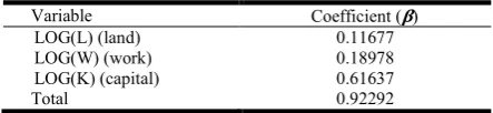
The returns to scale are obtained by adding the parameters β when there is a Cobb-Douglas function (Barbosa, 1985; Gujarati, 2006). The sum of the parameters β corresponding to the elasticities of the variables L, W and K indicated decreasing returns, as can be seen in Table 3.

Table 3. Parameters estimated by logarithmic multiple regression

Variable Coefficient ( )

LOG(L) (land) 0.11677

LOG(W) (work) 0.18978

LOG(K) (capital) 0.61637

Total 0.92292

Source: Research data. Based on IBGE (2010).

This result shows that the average production costs tend to increase as producers intensify the use of factors. In this perspective, the results show that new investments resulting in an intensified use of the factors should be planned based on a detailed economic feasibility study. It should be noted that there is the need for specific microeconomic studies that consider the specificities of each production system, whether developed on properties of micro, small, medium or large size, dealing with livestock or agriculture. It is also imperative to

develop and disseminate management practices and

technologies that enable higher average productivity. Otherwise, there may be producers’ indebtedness and economic infeasibility of activities.

Therefore, if this path is not changed and if new investments are not grounded on technical criteria, the competitive advantage of agriculture in Rio Grande do Sul will tend to be reduced.

AVERAGE PRODUCTIVITY OF FACTORS

The results of the calculation of average productivity show a gross output value of BRL 1,047.46 for each hectare used for agricultural activities. Similarly, the average production for each worker was BRL 16,108.95 and each unit of capital produced the equivalent to BRL 1.06 per year (Table 4).

Table 4. Average productivity (in BRL) of factors over GOV

Factor of

Production AP/year*

Minimum Productivity

Maximum Productivity L (land) 1,047.46 214.84 6,444.65 W (work) 16,108.95 7,772.00 44,806.86 K (capital) 1.0627 0.5028 1.7382 * Geometric mean. Source: Research data. Based on IBGE (2010).

The microregions with the best land productivity are Montenegro, Caxias do Sul, Lajeado-Estrela and Guaporé, with the two latter producing an amount equal or equivalent to BRL 2,500.00 / ha, while the microregions Campanha Ocidental, Jaguarão, Serras de Sudeste, Campanha Meridional and Campanha Central have the lowest productivity indicators, below BRL 390.00/ha. The measurement of work productivity showed a high standard deviation. The mostprominent microregions, with average work productivity above BRL 26,900.00/worker, are Campanha Ocidental, Vacaria, Jaguarão and Litoral Lagunar. In contrast, average work productivity in the microregions of Santa Rosa, Pelotas, Frederico Westphalen and Soledade was below BRL 10,000.00 in the year analyzed (Figure 2).

The capital factor of production also showed a high standard deviation. The farms of the microregions Vacaria, São Jerônimo, Campanha Ocidental and Ijuí had the best indicators, with average productivity above BRL 1.40.In contrast, in the microregions Campanha Central, Gramado-Canela, Caxias do Sul and Porto Alegre, theaverage productivity of capital was below BRL 0.70. With above-average productivity for the three factors, the most productive microregions are Carazinho, Camaquã, Ijuí, Montenegro, Não-Me-Toque, Passo fundo and São Jerônimo. Ranking second, with above-average productivity for two factors, are the microregions, Campanha Ocidental, Caxias do Sul, Cerro Largo, Cruz Alta, Guaporé, Jaguarão, Lajeado-Estrela, Litoral Lagunar, Osório, Sananduva, Santa Rosa, Santiago, Três Passos and Vacaria. In contrast, the microregions Cachoeira do Sul, Pelotas, Porto Alegre, Santa Maria and Soledadehad the lowest productivity for the three factors (Figure 3).

MARGINAL PRODUCTIVITY AND USE OF

RESOURCES

The results of the analysis of the marginal product of the

factors L, W and K used in the productive activities of farms

Source: Research data. Based on IBGE (2010).

Figure 3. Higher average productivity of factors of production used in farms, by microregion: Rio Grande do Sul

Source: Research data. Based on IBGE (2010).

Figure 4. Microregions

Based on IBGE (2010).

productivity of factors of production used in farms, by microregion: Rio Grande do Sul

Source: Research data. Based on IBGE (2010).

4. Microregions above-average factor productivity: Rio Grande do Sul

productivity of factors of production used in farms, by microregion: Rio Grande do Sul – 2006

GOV and c) the marginal productivity of capital confirms the

increase of BRL 0.66 in Q for every BRL 1.00 invested in the

infrastructure of farms (Table 5).

Table 5. Marginal productivity of factors (MP) over GOV

Factor of Production MP*

L (land) 122.31

W (work) 3,057.16

K (capital) 0.6550

*It is the derivative of output over factor, equivalent to: * MP = AP * βi

Source: Research data. Based on IBGE (2010).

MARGINAL RATE OF SUBSTITUTION (MRS)

Considering that the MRS of work over capital is equivalent to the ratio between the MP of work and the MP of capital, the replacement of one unit of skilled work requires the investment of BRL 4,667.49, (equation 11).

= =3.057,16

0,6550 = 4.667,49 (11)

Given these results, it is concluded that credit policies and exemptions that favor investment in farms is an alternative to expand production in the medium and long term. However, the decreasing returns to scale point to the need for policies that raise the competitiveness of the agricultural production in the Rio Grande do Sul. In this perspective, investments in infrastructure for irrigation; grain storage within the properties or in agricultural cooperatives, stables, milking parlors, milk coolers; construction of aviaries and piggeries, among others, tend to contribute to the diversification of production and increased income for farms in Rio Grande do Sul

Conclusions

The socioeconomic importance of agricultural production in Rio Grande do Sul has motivated this research. These activities not only generate jobs and income for many towns and cities, but also typically represent the state. However, due to adverse conditions arising from market issues and successive water stress episodes, they should be observed and stimulated carefully. Planning public policies should be preceded by structural and cyclical analyses. The production function was estimated in this context. The main results show that the ratios between product (Q) and factors (L,W, K) are increasing and that, overall, the properties that either have the largest area, are more work-intensive or have greater capital generate higher amount of product. Likewise, it was observed that the mere expansion of the area without investment in capital and technology does not usually result in significant growth of production. Conversely, stimulating investment and modernization can be a key element to promote the advancement of agricultural production and improve competitiveness indices, as long as guided by assessments of the economic viability of farms.

Thus, further microeconomic studies should consider the specific characteristics of each production system, and the use of econometric modeling to estimate the Cobb-Douglas function is one of the methodological alternatives for analysis. The validity of the results of this study can also be credited to census data. They not only accurately describe production, but were also a good fit to the model, because all parameters corroborated the economic theory and were statistically different from zero. Finally, if production is to be maximized, and the competitiveness of agricultural production of Rio Grande do Sul is to be maintained and increased, the government should adopt policies to stimulate investment, exempt the capital goods industry and strongly encourage the professionalization of farmers through rural extension activities and specific policies to address the bottlenecks of each activity.

REFERENCES

Barbosa, F. de H. 1985. Microeconomia: teoria, modelos

econométricos e aplicações à economia brasileira (Vol. 10). IPEA/INPES.

Brasil. 2009. Censo Agropecuário 2006. IBGE. Rio de

Janeiro, 2009. Disponible in<http://downloads.ibge.gov.br/ downloads_estatisticas.htm>. Accessible in. [last query in 16 September 2012].

Brasil. 2011. Contas regionais do Brasil: 2005-2009. Rio de

Janeiro, IBGE, Contas Nacionais n. 35.

Gujarati, D. N. 2006. Econometria básica. Elsevier Brasil.

Hoffmann, R. 2006. Análise de regressão: uma introdução à

econometria. São Paulo, Hucitec.

Ocergs-Organização das Cooperativas do estado do Rio

Grande do Sul. 2012. Expressão do cooperativismo

gaúcho: 2012 anto internacional das cooperativas. Porto

Alegre. Disponible in.<http://intranet.sescooprs.coop.br/ arquivos/arqs/20120719102955.pdf>. [last queryin 25 october 2012].

Santana, A. D. 2003. Métodos quantitativos em economia:

elementos e aplicações. Belém: Ufra.

Silva, L. A. C. 1996. A função de produção da agropecuária

brasileira: diferenças regionais e evolução no período

1975 – 1985. Doctoral dissertation, Escola Superior de

Agricultura Luiz de Queiroz, Piracicaba.

Soares, N. S., Silva, M. D. & Lima, J. E. D. 2007. A função de produção da indústria brasileira de celulose, em 2004.

Revista Árvore, 31(3), 495-502.

Solow, R. M. 1956. A contribution to the theory of economic

growth. The Quarterly Journal of Economics, 70(1), 65-94.

White, H. 1980. A heteroskedasticity-consistent covariance matrix estimator and a direct test for heteroskedasticity.

Econometrica: Journal of the Econometric Society,

817-838.

Varian, H. R. 2006. Microeconomia-princípios básicos. Elsevier Brasil