AN EMPIRICAL EVALUATION FOR THE INTRUSION DETECTION FEATURES BASED ON MACHINE LEARNING AND FEATURE SELECTION METHODS

6079

METHOD AND ALGORITHM FOR DIAGNOSTIC OF

EPILEPTIC EEG SIGNALS USING THE ADAPTIVE

ORTHOGONAL TRANSFORM

1_{ASMA HAFDI,} 2_{ABDENBI ABENAOU,} 3_{AHMED TOUMANARI}

1,2,3_{Laboratory of Systems Engineering and Information Technology (LiSTi), National School of Applied} Sciences, Ibn Zohr University, Agadir, Morocco

E-mail: 1_{[email protected],} 2_{[email protected],} 3_{[email protected]}

ABSTRACT

Electroencephalography (EEG) is one of the most used techniques for evaluating the functional status of the brain. It is essential for diseases’ diagnosis such as epilepsy. This pathology results from a cerebral dysfunction. The diagnosis of this pathology consists of detecting the appearance of paroxysmal activities in the EEG signals. The diagnostic of Epilepsy in EEG plays a crucial role in Computer Aided Diagnosis system (CAD). In this article, we suggest an approach based on the orthogonal adaptive transformation theory which makes it possible to extract the informative features of the EEG signals. The size of the vectors of the informative features obtained by this method is very short. This will allow to improve the quality of signals analysis and to increase their certainty of diagnosis

Keywords: Adaptive Orthogonal Transformation, Basis Functions, Extraction of the Informative Features

1. INTRODUCTION

The EEG is one of the main medical diagnostic tools [1]. The provided information on the bioelectric activity of the brain makes it possible to estimate not only the state of the nervous system but the whole organism as well. Electroencephalography (EEG) is widely used in neurology and it is essential for diseases diagnosis such as epilepsy [2]. This pathology results from a cerebral dysfunction which is noticed through repetitive and unpredictable brief crises.

Epileptic seizures are reflected in electroencephalogram (EEG) by the appearance of paroxysmal activities [3].

The diagnosis of this pathology therefore consists of detecting paroxysmal activities in the EEG signals of the patient. In diagnosis, the extracting of the informative features of the EEG signal is the most important step.

The analysis of the electroencephalogram signal (EEG) is quite complicated because of its no-stationary behavior [4].

The Karhunen-Loeve transformation [5] can be considered as an optimal mathematical

instrument for analyzing non-stationary signals. However, its practical use is limited because of the difficulty of calculating the singular functions of the covariance matrix of the signal to be analyzed and the absence of a fast transformation algorithm for the calculation of the spectrum.

To deal with these processes, the spectral methods based on conventional orthogonal transformations are often used (Fourier, Haar, Walsh,...) [6] thanks to the advantage of their fast algorithm of transformation. However, in the spectral domain these changes do not provide a higher distinction between the standard vector and the signal to be analyzed because of the enlargement of the obtained spectral. Therefore it is necessary for a spectral method to accurately detect this difference. If the features’ vector changes values in a considerable way from one class to another, this confirms the possibility of constructing an effective system for the diagnostic of signals. This is why the method of extraction of informative features constructs the most important phase in diagnosis.

6080 transformation operator to the standard vector of a class of the processed signals and to obtain a very short spectrum of informative characteristics.

This method improves the quality of analysis and increases the certainty of classification of EEG signals which leads to a better diagnosis of the state of the patient.

The aim is not to fully characterize the activities observed in the EEG signals. The pointed form, common to a large part of the paroxysmal activities, will be used as the main characteristic of the activities to be detected.

2. METHODS USED

The automatic detection of epileptic peaks in EEG was studied over the past 40 years [7],[8],[9]. Through the existing solutions, we distinguish essentially five types of techniques used in the domain of automatic detection of epileptic points:

2.1 Mimetic Techniques

These techniques attempt to reproduce the behavior of expert EEG readers (EEGers) to automatically detect the peaks. They compare characteristics established by the expert, such as the amplitude or duration of a wave with the characteristics of the processed signal. Peaks are detected by thresholding these criteria. The major disadvantage of this approach is that it detects events that are not peaks (for example cardiac artifacts or eye blinks may correspond to the same criteria as a peak).

2.2 Pattern Matching Techniques

These techniques consist in detecting points based on several points previously identified by an EEGer [10]. From these points, a pattern is constructed and is compared to the processed signal. The pattern can be a time representation, a frequency representation or a spatiotemporal representation of the peaks [11].

2.3 Parametric Techniques

These techniques assume that a signal that does not contain epileptic points is stationary, and the non-stationary of the signal reflects the presence of an epileptic points. Like mimetic techniques, this approach is sensitive to the presence of artifacts in the signal.

2.4 Neural Network Techniques

These techniques model signal processing tools; they are schematically close to the functioning of biological neurons. Several units

cooperate to form an assembly which, after training on different EEG signals containing epileptic points, is capable of detecting these points in any signal. In addition to the difficulty of defining a training database, the main complexity is to define the parameters at the input of the architecture of a neural network.

2.5 Spectral or Time-Frequency Analysis

This method consists in extracting information from the signal via its frequency representation. While some works use only Fourier transformation (to construct the spectrum which only presents the global frequencies of the signal), others exploit more elaborate Time-Frequency methods such as the wavelet transform [12]. They prove to be very effective in detecting epileptic points, but the choice of the wavelet to use is the major disadvantage of this approach.

3. METHOD AND ALGORITHM

In digital signal processing, the orthogonal linear transform of a signal X can be represented by the equation:

HX

N

Y



1

(1)

Where:

 H is the matrix operator of the transform size N x N whose number of rows corresponds to the number of basic functions to decompose the vector X.

 X = [x1, x2,……,xN]T is the original signal to transform having the size N = 2n_.

 Y = [y1, y2, …, yN]T is the vector of spectral coefficients calculated by the orthogonal spectral operator H of dimension N x N.

The process of calculation of the spectrum using Equation 1 requires N2 _{addition and} multiplication operations. The most effective means for reducing the number of operation is the rapid transformation algorithm (FFT) based on the method of Good [13] which consists of expressing the matrix operator H as a product of sparse matrices Gi composed by elementary matrices minimum dimension:

















)

cos(

)

sin(

)

sin(

)

cos(

)

(

, ,

, ,

, ,

j i j

i

j i j

i j

i j i

V











these are called spectral kernels.

6081

X

G

N

Y

n i

i

.

1

1







(2)

with:































2 , 2

, 1 ,

0

0

N i i

i i

V

V

V

G

_

where :

N

n



log

2 is the number of matrices Gi. So, each matrix Gi contains

2

N _{spectral kernels V}

i,j (ϕi,j) sized 2 х 2.

In the procedure of the adaptation of operator H to a class of signals (to be analyzed), the first step consists of calculating statistical characteristics (mean value in this case) of some signals recording for learning the classifier to form the class average vector Xm .

The synthesis of adaptive operator's basis functions H system is therefore based on average vector Xm. In other words, the operator of the transform is adapted to a class of signals represented by the average vector Xm if it replies to the following condition:

H

X

Y

_T



y

_c



t

N

,

0

,

,

0

1

1 m

a







(3)

where

Y

_T is the target vector, the first non-zero component yT,1, builds the adaptation criterion operator transform. Moreover, if the vectors are normalized, the Equation 3 becomes:





T

T

Y

X

H

N

1

,

0

,

,

0

1

m

a







(4) According to Parseval's relation, the

transform operator Ha is adaptive if the energy of the standard vector is concentrated in the first component of the target vector

Y

_T. The synthesis of adaptive operator Ha requires to determine the angular parameters



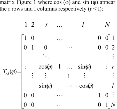
i,jof the spectral kernels Vi,j during the calculation of Gi . In [14], the Good’s matrix has a predetermined a fixed structure. The spectral kernels are arranged diagonally; the operator's synthesis is based on their kronecker’s product (the modified form). In this article, we suggest an approach based on the calculation of the angles of Givens’ rotation.

[image:3.612.314.515.113.301.2]

Let be Tr,l() the Givens’ rotation matrix Figure 1 where cos (φ) and sin (φ) appear at the r rows and l columns respectively (r < l):

Figure 1: Representation of the Givens’ rotation matrix

The matrices Gi are calculated using the product of matrices _,j

(

_i,j

)

l r

T



:

)

(

_,

2 /

1 , 2

j i N

j i

j j

i

T

n i

G





 





₍₅₎

The calculation of the target vector YT can be achieved step by step using the matrix Gi with an iterative procedure using the following recursive relation:

1





i i i

G

Y

Y

where:

i = 1 …log2 N and Y0 = Xm

The angular parameters



i,j of the

matrices j l r

T

_, are calculated according to the components of the vector Yi-1 by the following relation:

. 2 1 , 1

, 0 0

,

, 1 2

, 1 ,

, 1 2 , 1 ,

N j

n i

y y

si y y arctg

j i j

i j

i

j i

j i j

i

i n

i n



 

      

  

    

   

 

 

 

 

 

(6)

To clarify the idea of the algorithm, we consider the following example of the calculation of the transform operator size N = 4.

N l r T_rl

  

 

  



 





 

2 1

1 0 0

0

0 1 0

0

) cos( )

sin(

1

) sin( 1

) cos(

0 0 0

1 0

0 0 0

1

) ( ,

          

 

          

 

 











6082 Lets be

X

_m





x

_m,1

,

x

_m,2

,

x

_m,3

,

x

_m,4



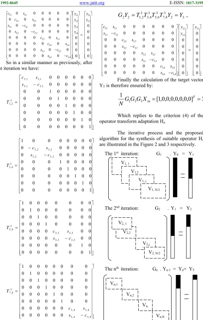
Tthe vector standard.

In the first iteration i = 1, we will calculate the matrices , 1 0 0 0 0 0 0 0 0 1 0 0 0 0 0 0 0 0 1 0 0 0 0 0 0 0 0 0 0 0 0 0 0 0 1 0 0 0 0 0 0 0 0 1 0 0 0 0 0 0 0 0 1 0 0 0 0 0 0 0 1 , 1 1 , 1 1 , 1 1 , 1 1 5 , 1                             c s s c T , 1 0 0 0 0 0 0 0 0 1 0 0 0 0 0 0 0 0 0 0 0 0 0 0 0 1 0 0 0 0 0 0 0 0 1 0 0 0 0 0 0 0 0 1 0 0 0 0 0 0 0 0 0 0 0 0 0 0 0 1 2 , 1 2 , 1 2 , 1 2 , 1 1 6 , 2                             c s s c T , 1 0 0 0 0 0 0 0 0 0 0 0 0 0 0 0 1 0 0 0 0 0 0 0 0 1 0 0 0 0 0 0 0 0 1 0 0 0 0 0 0 0 0 0 0 0 0 0 0 0 1 0 0 0 0 0 0 0 0 1 3 , 1 3 , 1 3 , 1 3 , 1 1 7 , 3                             c s s c T , 0 0 0 0 0 0 0 1 0 0 0 0 0 0 0 0 1 0 0 0 0 0 0 0 0 1 0 0 0 0 0 0 0 0 0 0 0 0 0 0 0 1 0 0 0 0 0 0 0 0 1 0 0 0 0 0 0 0 0 1 4 , 1 4 , 1 4 , 1 4 , 1 1 8 , 4                             c s s c T with:

ci,j=cos(i,j) and si,j=sin(i,j).

Using the Equation 6, we calculate the parameters i,j, and we obtain:

                                                                                   0 0 0 0 0 0 0 0 0 0 0 0 0 0 0 0 0 0 0 0 0 0 0 0 0 0 0 0 0 0 0 0 0 0 0 0 0 0 0 0 0 0 0 0 0 0 0 0 0 0 0 0 4 , 1 3 , 1 2 , 1 1 , 1 et,8 et,7 et,6 et,5 et,4 et,3 et,2 et,1 4 , 1 4 , 1 3 , 1 3 , 1 2 , 1 2 , 1 1 , 1 1 , 1 4 , 1 4 , 1 3 , 1 3 , 1 2 , 1 2 , 1 1 , 1 1 , 1 y y y y r r r r r r r r c s c s c s c s s c s c s c s c

For the second iteration i = 2, we calculate the parameters



_i,j in an analogous manner, from the vector Y1 which will determine the matrices:

, 1 0 0 0 0 0 0 0 0 1 0 0 0 0 0 0 0 0 1 0 0 0 0 0 0 0 0 1 0 0 0 0 0 0 0 0 1 0 0 0 0 0 0 0 0 0 0 0 0 0 0 0 1 0 0 0 0 0 0 0 1 , 2 1 , 2 1 , 2 1 , 2 2 3 , 1                             c s s c T                             1 0 0 0 0 0 0 0 0 1 0 0 0 0 0 0 0 0 1 0 0 0 0 0 0 0 0 1 0 0 0 0 0 0 0 0 0 0 0 0 0 0 0 1 0 0 0 0 0 0 0 0 0 0 0 0 0 0 0 1 2 , 2 2 , 2 2 , 2 2 , 2 2 4 , 2 c s s c T , 1 0 0 0 0 0 0 0 0 0 0 0 0 0 0 0 1 0 0 0 0 0 0 0 0 0 0 0 0 0 0 0 1 0 0 0 0 0 0 0 0 1 0 0 0 0 0 0 0 0 1 0 0 0 0 0 0 0 0 1 3 , 2 3 , 2 3 , 2 3 , 2 2 7 , 5                             c s s c T                             4 , 2 4 , 2 4 , 2 4 , 2 2 8 , 6 0 0 0 0 0 0 0 1 0 0 0 0 0 0 0 0 0 0 0 0 0 0 0 1 0 0 0 0 0 0 0 0 1 0 0 0 0 0 0 0 0 1 0 0 0 0 0 0 0 0 1 0 0 0 0 0 0 0 0 1 c s s c T

The decomposition of the vector Y1 gives:

)

(

_,

, i j j

l r

6083                                                                                    0 0 0 0 0 0 0 0 0 0 . 0 0 0 0 0 0 0 0 0 0 0 0 0 0 0 0 0 0 0 0 0 0 0 0 0 0 0 0 0 0 0 0 0 0 0 0 0 0 0 0 0 0 0 0 0 0 0 0 2 , 2 1 , 2 4 , 1 3 , 1 2 , 1 1 , 1 4 , 2 4 , 2 3 , 2 3 , 2 4 , 2 4 , 2 3 , 3 , 2 2 , 2 2 , 2 1 , 2 1 , 2 2 , 2 2 , 2 1 , 2 1 , 2 y y y y y y c s c s s c s c c s c s s c s c é

So in a similar manner as previously, after the last iteration we have:

                            1 0 0 0 0 0 0 0 0 1 0 0 0 0 0 0 0 0 1 0 0 0 0 0 0 0 0 1 0 0 0 0 0 0 0 0 1 0 0 0 0 0 0 0 0 1 0 0 0 0 0 0 0 0 0 0 0 0 0 0 1 , 3 1 , 3 1 , 3 1 , 3 3 2 , 1 c s s c T                              1 0 0 0 0 0 0 0 0 1 0 0 0 0 0 0 0 0 1 0 0 0 0 0 0 0 0 1 0 0 0 0 0 0 0 0 1 0 0 0 0 0 0 0 0 0 0 0 0 0 0 0 0 0 0 0 0 0 0 1 2 , 3 2 , 3 2 , 3 2 , 3 3 4 , 3 c s s c T                             1 0 0 0 0 0 0 0 0 1 0 0 0 0 0 0 0 0 0 0 0 0 0 0 0 0 0 0 0 0 0 0 1 0 0 0 0 0 0 0 0 1 0 0 0 0 0 0 0 0 1 0 0 0 0 0 0 0 0 1 3 , 3 3 , 3 3 , 3 3 , 3 3 6 , 5 c s s c T                             4 , 3 4 , 3 4 , 3 4 , 3 3 8 , 7 0 0 0 0 0 0 0 0 0 0 0 0 0 0 1 0 0 0 0 0 0 0 0 1 0 0 0 0 0 0 0 0 1 0 0 0 0 0 0 0 0 1 0 0 0 0 0 0 0 0 1 0 0 0 0 0 0 0 0 1 c s s c T

The Y3 vector is obtained by:

,

3 2 3 8 , 7 3 6 , 5 3 4 , 3 3 2 , 1 2

2

Y

T

T

T

T

Y

Y

G





                                                                                   0 0 0 0 0 0 0 0 0 0 0 0 0 . 0 0 0 0 0 0 0 0 0 0 0 0 0 0 0 0 0 0 0 0 0 0 0 0 0 0 0 0 0 0 0 0 0 0 0 0 0 0 0 0 0 0 0 0 0 0 0

0 3,1

2 , 2 1 , 2 4 , 3 4 , 3 4 , 3 4 , 3 3 , 3 1 , 3 3 , 3 3 , 3 2 , 3 2 , 3 2 , 3 2 , 3 1 , 3 1 , 3 1 , 3 1 , 3 y y y c s s c c s s s c s s c c s s c

Finally the calculation of the target vector YT is therefore ensured by:

,

]

0

,

0

,

0

,

0

,

0

,

0

,

0

,

1

[

1

m 3 2 1 T T

Y

X

G

G

G

N





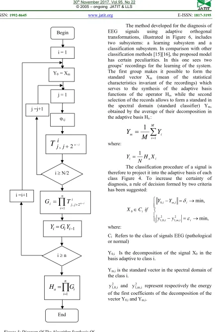
Which replies to the criterion (4) of the operator transform adaptation Ha.

[image:5.612.114.521.73.712.2]

The iterative process and the proposed algorithm for the synthesis of suitable operator Ha are illustrated in the Figure 2 and 3 respectively.

Figure 2: Iterative Procedure Of Good’Matrix

The nth _{iteration: G}

n . Yn-1 = Yn= YT

Vn, Vn,N Vn,2

Vn,1

The 1st _{iteration: G}

1 . Y0 = Y1 V1, 1

V1,2 V1, j

V1, N/2

V2,2

The 2nd _{iteration: G}

2 . Y1 = Y2

V2,j

H _V

[image:6.612.96.539.48.716.2]

6084

Figure 3: Diagram Of The Algorithm Synthesis Of Adaptive Orthogonal Transformation Operator

The method developed for the diagnosis of EEG signals using adaptive orthogonal transformations, illustrated in Figure 6, includes two subsystems: a learning subsystem and a classification subsystem. In comparison with other classification methods [15][16], the proposed model has certain peculiarities. In this one sees two groups’ recordings for the learning of the system. The first group makes it possible to form the standard vector Xm (mean of the statistical characteristics invariant of the recordings) which serves to the synthesis of the adaptive basis functions of the operator Ha, while the second selection of the records allows to form a standard in the spectral domain (standard classifier) Ym, obtained by the average of their decomposition in the adaptive basis Ha :







M i

i

m

Y

M

Y

1

1

where:

i i H X

N

Y  1 _a

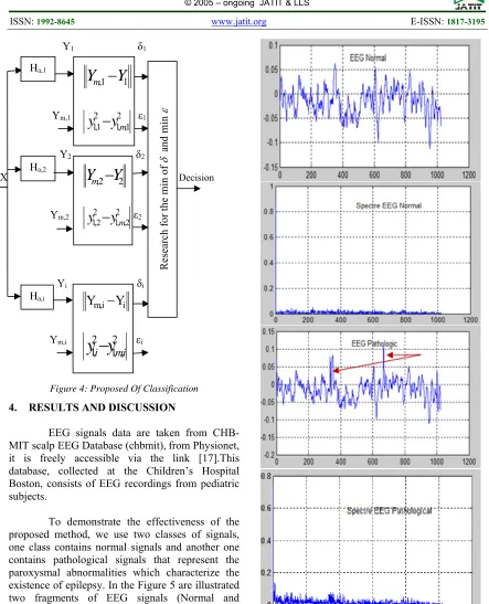
The classification procedure of a signal is therefore to project it into the adaptive basis of each class Figure 4. To increase the certainty of diagnosis, a rule of decision formed by two criteria has been suggested:

     

  

   

min, min,

2 , , 1 2

, 0 , 1

, , 0

0

i i m i

i i m i

i

y y

Y Y

if C X

 

where:

Ci Refers to the class of signals EEG (pathological or normal)

Y0,i Is the decomposition of the signal X0 in the basis adaptive to class i.

Ym,i is the standard vector in the spectral domain of the class i.

2 i, 0 , 1

y and 2

i, m , 1

y represent respectively the energy of the first coefficients of the decomposition of the vector Y0,i and Ym,i.

End







n

i i

a

G

H

1 i  n

1





_{i i}

i

G

Y

Y

i =i+1

φi,j

i  N/2 j =j+1

Y0 = Xm i = 1

j = 1 Begin

i

j

j

n i

T

_,

_

₂





 





n

i i

j j i

T

n i

G

[image:7.612.82.525.59.606.2]

6085

Figure 4: Proposed Of Classification

4. RESULTS AND DISCUSSION

EEG signals data are taken from CHB-MIT scalp EEG Database (chbmit),from Physionet, it is freely accessible via the link [17].This database, collected at the Children’s Hospital Boston, consists of EEG recordings from pediatric subjects.

To demonstrate the effectiveness of the proposed method, we use two classes of signals, one class contains normal signals and another one contains pathological signals that represent the paroxysmal abnormalities which characterize the existence of epilepsy. In the Figure 5 are illustrated two fragments of EEG signals (Normal and pathological EEG) and their projections in adaptive basis.

[image:7.612.315.520.68.620.2]

Thanks to the selectivity of the transform, the aspects of the Yi spectra of the informative features are clearly distinguished. The presence of a peak (epileptic point) in the signal causes a sharp variation in the spectrum. This leads to a better classification and a diagnosis with a high certainty.

Figure 5: Calculation Of The Spectrum Of EEG Signals Using Adaptive Basis Functions

5. CONCLUSION

In this approach, the resolution of the problem of biological signals diagnosis is based on the use of the adaptive orthogonal transform whose functions can be set according to the data to be Ym,i εi

i i, m

Y

Y



2 ,, ,1 2

,1i

y

mi

y



X Decision

Ha,i

Yi δi Y2 δ2 Ha,2

2 2

,

Y

Y

_m



2 2 , , 1 2

2 , 1

y

m

y



Ym,2 ε2 Ym,1 ε1

Research f

or

the min

of



a

nd min



Y1 δ1

1 1

,

Y

Y

_m



2 1 , ,1 2

1 ,1

y

m

y



6086 analyzed. This approach has helped to develop a method of identification in which the property is used in the selectivity of the conversion and reached a high distinction of vector features of signals.

The major advantage of this method lies in the possibility of adapting the operator of the transform to the standard vector of a class of the given signals; this allows extracting a vector of the most relevant features from the signals.

The proposed approach cannot be used in unsupervised classification where signal classes are unknown. In fact, the synthesis of the operator adaptable to a given class requires prior information on the signals of the class that we can obtain by the calculation of one of the statistical characteristics which are invariant at the moment of emission of the signal (correlation, energetic spectrum and others).

The obtained results in this article allow drawing a conclusion about the prospect of the application of the methodology developed for the resolution of various problems such as classification, identification, technical and medical diagnostic and pattern recognition. It may be noted that this method can be projected on low variable signals related applications, that is to say the spectral shape signals in the low frequencies.

REFRENCES:

[1] J.M. Guérit, D. Debatisse, “Neurophysiological bases and principles of electroencephalogram interpretation in the intensive care unit”, Réanimation, Vol. 16, 2007, pp. 546-552. [2] Abeg Kumar Jaiswal, Haider Banka, “Epileptic

seizure detection in EEG signal with GModPCA and support vector machine”, Bio-Medical Materials and Engineering, Vol. 28, 2017, pp. 141-157.

[3] Samuel Boudet, “Filtrage d'artefacts par analyse multicomposante de l'électroencéphalogramme de patients épileptiques”, Thesis, Laboratory of Automatic, Computer Engineering and Signal, Lille Catholic University, July, 2008, pp. 34-36. [4] Abdulhamit Subasi, “Application of Classical

and Model-Based Spectral Methods to Describe the State of Alertness in EEG”, Journal of Medical Systems, Vol. 29, No. 5, October, 2005, pp. 473-486.

[5] Stefanos K. Goumas, Michael. E. Zervakis, G. S. Stavrakakis, “Classification of Washing

Machines Vibration Signals Using Discrete Wavelet Analysis for Feature Extraction”,

IEEE Instrumentation and Measurement

Society, Vol. 51, No. 3, June, 2002, pp. 497-508.

[6] B.J. Falkowski, S. Rahardja, “WaIsh-like functions and their relations”, IEE Proc.-Vis. Image Signal Process., Vol. 143, No. 5, October, 1996, pp. 279-284.

[7] J.R.G. Carrie, “A technique for analyzing

transient EEG abnormalities”,

Electroencephalography and Clinical Neurophysiology, Vol. 32, No. 2, February, 1972, pp. 199-201.

[8] Gevins, A.S, Yeager, CL, Diamond, S.L, Spire, J.P, Zeitiin, G.M. & Gevins, A.H, “Automated analysis of the electrical activity of the human brain (EEG): A progress report”, IEEE Proc, Vol. 63, No. 10, 1975, pp. 1382-1399.

[9] J. Gotman, P. Gloor, “Automatic recognition of inter-ictal epileptic activity in the human scalp EEG recordings”, Electroencephalography and clinical neurophysiology, Vol. 41, 1976, pp. 513-529.

[10]

Goelz, H, Jones, R.D. & Bones, P.J, “Wavelet

analysis of transient biomedical signals and its application to detection of epileptiform activity in the EEG”, Clinical Electroencephalography, Vol. 31, 2000, pp. 181 -191.

[11] Pascal Viot, “Cours de Modélisation Dynamique et Statistique des systèmes Théorique des liquides”, Laboratory of Physics Theoretical of Liquids, Paris, 2009.

[12] Lotfi Senhadji, Fabrice Wendling, “Epileptic transient detection: wavelets and time-frequency approaches”, Clinical Neurophysiology, Vol. 32, No. 3, June, 2002,pp. 175-192.

[13] I.J. Good, “The factorization of sum of matrices and the multivariate cumulants of a set of

quadratic expressions”, Journal of

Combinatorial Theory, Series A, Vol. 11, July, 1971, pp. 27-37.

[14] Abenaou Abdenbi, “Development of a method for the synthesis of adaptive spectral operators for the analysis of random signal”, International Journal of Computer Theory and Engineering (IJCTE), Vol. 9, No. 3, 2016.

6087 [16] A. Subasi, “EEG signal classification using

wavelet feature extraction and a mixture of

expert model”, Expert Systems with

Applications, Vol. 32, No. 4, 2007, pp. 1084– 1093.

[image:10.612.96.518.111.438.2]

6088

Figure 6: Proposed System Of Diagnostic

Classification Sub-system

Decision Signal EEG to

be classified

Extraction of the features Set 2

Set 1

EEG

Pat

hol

ogi

cal

Calculation of the spectral standard vector

Ym,2 Synthesis of the

operator for class pathological Ha,2 Formation of

the standard vector of the class 1 Xm,2 Formation of

the standard vector of the class 1 Xm,1

Synthesis of the operator for

class normal Ha,1

Calculation of the spectral standard

vector Ym,1

Set 2

Ex

traction

o

f statistica

l ch

aract

eristics (Correlatio

n,

mean va

lu

e)

Set 1

EEG _Normal