RULES REDUCTION AND OPTIMIZATION OF FUZZY LOGIC MEMBERSHIP FUNCTIONS FOR INDUCTION MOTOR SPEED CONTROLLER

5058

OPTIMIZATION OF PID CONTROLLER USING GENETIC

ALGORITHM FOR MISSILE’S AUTOMATIC STEERING

SYSTEM

1_{MOHAMMAD ISA IRAWAN,} 2_{IMAM MUKHLASH,} 3_{FEDRIC FERNANDO}

1,2,3_{Department of Mathematics, Institut Teknologi Sepuluh Nopember, Indonesia}

E-mail: 1_{[email protected],} 2_{[email protected],} 3_{[email protected]}

ABSTRACT

Missile’s steering system is one of systems that use Proportional Integral Derivative (PID) controller. The difficulty in using this controller is tuning the parameters, because PID controller uses 3 controllers. There are a lot of different ways to get values of the controller’s parameters, such as using classical method or even using evolutionary algorithms. One of evolutionary algorithms is Genetic Algorithm (GA). GA is a search algorithm that is based on genetic principles and usually used in optimizing systems. In this research, performance of the controller that is obtained using GA and using conventional method (i.e. Ziegler-Nichols (Z-N)) are compared in order to optimize missile’s steering system. The result of the simulation shows that PID controller obtained using GA is faster in making the system going towards the setpoint than PID controller obtained using Z-N method. Furthermore, parameters of PID controller from GA make system more robust than parameters from Z-N.

Keywords: Parameter Optimization, PID Controller, Ziegler-Nichols, Genetic Algorithm (GA)

1. INTRODUCTION

Proportional Integral Derivative (PID) controller is commonly used to get the optimum solution, because it’s gives better efficiency. In order to get this efficiency, real output should be the same as the output that had been set. Therefore, controller is one of the tools that must be prepared. Missile’s steering engine is one of systems that use PID controller to find its optimum solution. PID controller used to control the position of missile’s fins, that will affect the missile’ direction. By positioning the fins in the correct place faster, the use of fuel will be reduced. Recently, a high-tech missile should have a robust, smart, and accurate system [1]. That is why controller is needed.

Difficulty in using PID controller is how to tune the parameters [1]. There are a lot of methods that used to tune the parameters, for example, classic methods that still commonly used such as Ziegler-Nichols oscillation method, Ziegler-Ziegler-Nichols reaction curve method, Cohen-Coon reaction curve method, etc. Recent show that there is a drastic improvement in tuning if using evolutionary algorithm [1][3]. This algorithm gives a better solution for each iteration.

Genetic Algorithm (GA) is an evolutionary algorithm that uses evolutionary genetic as its algorithm’s model. GA is one of artificial intelligent

method which commonly used in a problem that needs an optimal solution by correcting itself. GA usually used in many applications, such as, optimization, scheduling, sorting, etc. [1]-[5]

In this paper, classical method Ziegler Nichols and Genetic Algorithm will be compared in optimize the parameters of PID controller in a missile’s steering system. The rise time, peak time, maximum overshoot, and settling time of the output will be compared to see which method is better. Beside of that, we’ll add constant and random disturbances to the system in order to compare these methods.

2. LITERATURE REVIEW

Genetic Algorithm is proved to solved some problems, such as PID parameters optimization [1]-[3], vehicle routing problem [4], multi-objective optimization[5], and many else. Genetic Algorithm is used to optimize because its ability to improve itself for each iteration, improvement in Genetic Algorithm depends on its fitness value. Fitness value from one problem and another maybe different, but it can be same. Even in same problem, several different fitness will show the difference [3].

5059 iteration is going bigger [1]-[3]. One of system that usually uses PID controller is missile’s control system [1][2]. The value of PID applied to system, to make the system going toward desired output, intended to be more accurate, faster, and more robust than system without PID controller.

In this paper, PID parameters will be generated by using Z-N method and Genetic Algorithm with several fitness values, PID parameters will optimize the missile’s control system. Controlled system will be checked by its overshoot, settling time, rise time, peak time, error steady state, and by adding some disturbances. We will only use the simulation of model in order to try the effectiveness of the PID that generated by Z-N and GA towards the system’s model.

3. SYSTEM MODEL

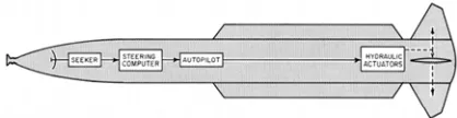
The altitude of the missile should be controlled so the actual position is manipulated in such a way to make the missile is going toward the desired position [1]. Therefore, to make sure that missile’s position can be changed at will, a controller will be needed, in this case the controller is PID controller. For example, a simple missile can be seen in Fig. 1[6]

Figure 1: Terrier (HT-3) Guidance and Control System

In Fig. 1, the guidance system starts from seeker, steering computer, and autopilot. For the control system or the steering system, this type of missile only has hydraulic actuators.

The hydraulic actuator will control the fin, to get its position right. The position of fin will determine the direction of the missile. In this paper, we will optimize fin’s mathematical model.

By using the second law of Newton, we can write that the force in the fin is:

(1)

Where:

a = acceleration

c = damping coefficient of the fin k = spring constant

m = mass

v = velocity x = position

And if we want to move the fin faster, we add another force to the fin, so the Equation (1) will change to:

Where: u = added force

Natural frequency is the frequency of free vibration system [7]. That’s mean that natural frequency is the frequency when the system oscillates without external force. Natural frequency is defined as [7]:

Where:

= natural frequency

Critical damping is the minimum viscous damping that will allow a displaced system to return to its initial position without oscillation. Critical damping is defined as [7]:

2√

2

2

Where:

= critical damping

The ratio between the damping coefficient and critical damping is called damping ratio or fraction of critical damping [7]. Defined as:

Where:

5060 By using natural frequency, critical damping, and damping ratio that defined above, we can get that the acceleration will change to:

2 (2)

Assuming as position, as velocity, as acceleration, and the output is the position of the fin. From Equation (2), the state space of the model will be:

0 1

2 0

1 0

The transfer function of the missile can be obtained by processing the state space that we get earlier. Let’s assume that:

0 1

2 0

1 0 0

Transfer function can be obtained by calculating matrixes from state space:

Therefore, we can get the transfer function of the missile’s steering system in order two function [1][2][8]:

1

1 1 _{2 1}

Where:

= Transfer Function of missile’s steering system.

We assume that 0.01 and 0.7, therefore we can get that the transfer function is [1][2]:

1

0.01 2 2 0.01 ∗ 2 ∗ 0.7 1

1

0.0001 0.014 1

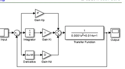
After that, model in Simulink will be created with the transfer function and the PID controller. The model of that system is in Fig. 2.

Figure 2: Plant System with PID Controller

We will now add the PID parameter, by using Z-N method and by using GA we will replace gain Kp, Ki, and Kd in Fig. 2, and then compare the result. Values that we’ll compare are rise time, peak time, maximum overshoot, settling time, and error steady state.

Rise time is time needed for the system to reach its setpoints. Peak time is time for the system to reach its peak. Maximum overshoot, is the maximum error value, from the peak of the amplitude to its setpoints. Settling time is time needed for the system to go in the error band, error band usually defined to be some percentage of the setpoints.

Beside of that, we will test the model by adding some disturbances, uniform and random disturbance. The purpose is to compare the robustness of the system that added with PID from Z-N and GA towards some disturbances.

4. OPTIMIZATION USING Z-N METHOD

4.1.Optimization using Z-N method

In this process, parameters of PID controller will be get by the help of SISO tool MATLAB. First, we should input the transfer function of the system. And then, with that transfer function, we’ll run the SISO tool. We get the compensator:

0.00834 5.06 766.68

With the parameter of PID:

5.06 766.68

0.00834

5061

4.2.Analysis of Optimization Using Z-N Method

By using model in Fig. 3, the outcome graph from the system can be seen in Fig. 4.

Figure 4: Graph of Output System with Z-N Method

From output in Fig 4, we get that the rise time from 0% to 90%, the peak time, maximum overshoot, and the settling time in Table 1

Table 1: Output System with Z-N Method

Parameter Value

Rise Time 0.0064 second Peak Time 0.0 131 second Maximum Overshoot 48.7842% Settling Time 0.0737 second Error Steady State 1.999e-13% 

5. OPTIMZATION USING GENETIC

ALGORITHM

5.1.Genetic Algorithm in General

Genetic Algorithm is a searching technique in computer science for searching the estimation of solution for optimizing and searching problem. Genetic Algorithm is a special class from evolutionary algorithm that using technique inspired by evolutionary in biology, like inheritance,

mutation, nature selection, and recombination (crossover).

Genetic Algorithm in general requires two things to be defined: (1) genetic representation from the solution, (2) function that has capability to evaluate it [9].

In simple ways, general algorithm from genetic algorithm can be done in 5 steps:

1. Generating an individual population with random population as initial population.

2. Evaluate the fitness for each individual with the desired output.

3. Choose the individual with the high match rate and eliminate the others.

4. Reproduction, makes a crossover for each selected individual, and then does a mutation.

5. The new population is generated and repeat step 2 – 4 until the desired solution is founded or until the limit of the iterations is fulfilled.

5.2.Optimization in Using Genetic Algorithm

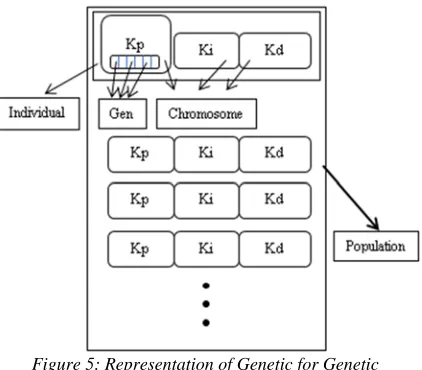
This process is a process where the value of controller P, controller I, and controller D will be searched by using genetic algorithm. In this case, an individual will contain 3 chromosomes. Each chromosome will be the value of Kp, Ki, and Kd. Each Kp, Ki, and Kd will be a real number, and gen will contain the binary from that number. In Fig 5, we can see the illustration of representation of genetic for Genetic Algorithm.

Figure 5: Representation of Genetic for Genetic Algorithm

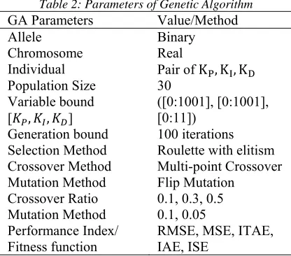
5062 Table 2: Parameters of Genetic Algorithm

GA Parameters Value/Method

Allele Binary

Chromosome Real

Individual Pair of K , K , K

Population Size 30 Variable bound

[ , , ]

([0:1001], [0:1001], [0:11])

Generation bound 100 iterations Selection Method Roulette with elitism Crossover Method Multi-point Crossover Mutation Method Flip Mutation Crossover Ratio 0.1, 0.3, 0.5 Mutation Method 0.1, 0.05 Performance Index/

Fitness function RMSE, MSE, ITAE, IAE, ISE

5.2.1. Initialization

As declared in Table 2, the variable bound of the Kp, Ki, and Kd are 0 to 1001, 0 to 1001 and 0 to 11. The value of Kp, Ki, and Kd will be randomize but will still in that boundary.

5.2.2. Evaluation

Evaluate the fitness value, each individual will be evaluated by using its fitness value. Fitness value will determine with individual is better than the others. Fitness value in this optimization is described as [3]:

1

Value of error in the optimization will be using RMSE (Root Mean Squared Error), MSE (Mean Squared Error), ITAE (Integral of Time Absolute Error), IAE (Integral of Absolute Error), and ISE (Integral of Squared Error).

Because the data that we process are discrete, error function that we used will be:

1

1

| |

| |

Where:

= error in time

5.2.3. Selection

Selection is the early stage of reproduction, selection will be select the individual that will be processed for next generation. In this paper, selection will be using roulette machine method. The fitness value of each individual will be its percentage to be selected for next generation. After we get the percentage from each individual, we then spin the roulette and select individual that selected by roulette as the parent of next generation.

Beside of that, elitism will be used to make sure that the next gen will be better for each iteration. Elitism is a method of selecting best individuals to be brought in the next gen. Such individuals can be lost if they are not selected or if they are changed because of mutation [10]. In this case, only the best individual will be brought to the next gen.

5.2.4. Crossover

After we get the individuals from selection, the next step is using them as the parent of the next generation. Crossover in this step will be using binary crossover.

First, we randomly select 2 individuals from the selected individuals as parent for the one of the next generation. Each chromosome from the parent individual will changed to a binary number, for chromosome of Kp in parent 1 will be crossover with chromosome of Kp in parent 2, chromosome of Ki in parent 1 will be crossover with chromosome of Ki in parent 2, and chromosome of Kd will be crossover with chromosome of Kd in parent 2.

Second, we select some of the points or locations of the gen in the chromosome, and then switch the value in the selected gen from each parent. The result will be the individuals of the next generation.

5.2.5. Mutation

5063

5.3.Analysis of Optimization Using Genetic

Algorithm

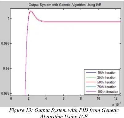
By using the parameters and method in Table 2, we can get the value of Kp, Ki, and Kd by each performance indexes. After several times of trial, we pick the best fitness value that generated from each performance indexes. First, the fitness value for each generation by using RMSE shown in Fig. 6.

Figure 6: Fitness Value Using RMSE for Each Generation

In Fig. 6, we can see how the fitness value grows in each iteration. We select the value of Kp, Ki, and Kd in 10th _{generation, 25}th _{generation, 50}th

generation, 75th _{generation, and 100}th _{generation, as}

in Table 3.

Table 3: Best Value of PID Controller’s parameters from Genetic Algorithm using RMSE

Iteration P I D Fitness

10 299.3178 36.6431 0.2436 38.5319 25 299.3178 338.1776 0.2436 38.7382 50 987.8833 0 0.2436 52.2668 75 987.8833 0 0.2436 52.2668 100 987.8833 901.0611 0.2436 52.3153

The value of Kp, Ki, and Kd from Table 3 then will be inserted to the model, and the output will be compared. The graph of the output shown in Fig. 7 and the value of the output shown in Table 4.

As we see in Table 4 and Fig. 7, we can conclude that the output of the system will become more fast in the rise time and peak time, yet become slower in getting the settling time, and the overshoot is become worst in each generation. The error steady state of the system in each generation having fluctuation.

Table 4: Output System with PID from Genetic Algorithm with RMSE

Iteration Rise Peak Overshoot Settling ESS(%) 10 0.0018 0.0028 1.88 % 0.0020 0.2855 25 0.0018 0.0028 1.97 % 0.0020 0.0766 50 0.0008 0.0012 22.61 % 0.0024 0.1011 75 0.0008 0.0012 22.61 % 0.0024 0.1011 100 0.0008 0.0012 22.65 % 0.0024 0.0309

Figure 7: Output System with PID from Genetic Algorithm with RMSE

Next, we check the fitness value for each generation by using MSE that can be found in Fig. 8. As we see in Fig. 8, the fitness value sharply raises at generation 6-7. Like RMSE, we pick 10th_{, 25}th_,

50th_{, 75}th_{, and 100}th _{generation as in Table 5, to}

compare the output.

Table 5: Best Value of PID Controller’s parameters from Genetic Algorithm using MSE

Iteration P I D Fitness

5064 Figure 8: Fitness Value Using MSE for Each Generation

The value of Kp, Ki, and Kd from Table 5 then will be inserted to the model, like value of RMSE before, and the output will be compared. The graph of the output shown in Fig. 9 and the value of the output shown in Table 6.

Figure 9: Output System with PID from Genetic Algorithm with MSE

Table 6: Output System with PID from Genetic Algorithm with MSE

Iteration Rise Peak Overshoot Settling ESS(%) 10 0.0009 0.0013 19.64 % 0.0020 0.1278 25 0.0008 0.0012 23.77 % 0.0025 0.0286 50 0.0008 0.0012 16.72 % 0.0018 0.0279 75 0.0008 0.0012 16.72 % 0.0018 0.0279 100 0.0008 0.0012 16.72 % 0.0018 0.0262

As we see in Table 6 and Fig. 9, we can conclude that the output of the system will become more fast in the rise time, peak time, and settling time for each iteration. The overshoot gets some fluctuation, yet become better for next iteration. The value of error steady state getting better for every iteration.

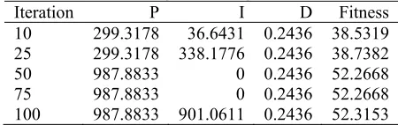
Next, we see for the PID parameters and their fitness value using ITAE, the graph of fitness value using ITAE can be found in Fig. 10. The value of fitness sharply raises from the second of GA starts, at first iteration and doesn’t change until 100th

iteration.

Figure 10: Fitness Value Using ITAE for Each Generation

In Table 7, we pick PID parameters from 10th

generation, 25th _{generation, 50}th _{generation, 75}th

generation, and 100th _{generation, and as we}

expected, the value of PID is same, because of the fitness value doesn’t change from early iteration. Therefore, in Fig. 11, we can see that the graph of the outputs is overlapping each other.

Table 7: Value of PID Controller’s parameters from Genetic Algorithm using ITAE

Iteration P I D Fitness

5065 Figure 11: Output System with PID from Z-N Method

and Genetic Algorithm

The output system that generated by using PID value from GA that using ITAE, we get the rise time, from 0% to 90% is 0.004 seconds. The peak time, or the time that system need to go to its amplitude’s highest peak is 0.0069. Maximum value of its overshoot is 1.51% from the desired output. The system started to getting in the 5% error of the output in 0.0045 seconds, with its error steady state 0.00000052% of the output.

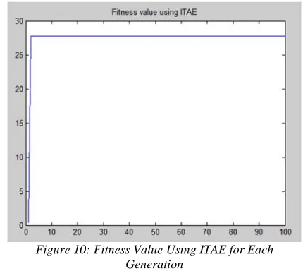
Following ITAE, next we check the result using IAE as part of the value fitness. In Fig. 12, we see that in generation 50 to generation 51, there’s the only change of the fitness value in the experiment, from 0.0871 to 0.1007.

Figure 12: Fitness Value Using IAE for Each Generation

Same as before, we select the value of PID parameters in 10th_{, 25}th_{, 50}th_{, 75}th_{, and 100}th

generation. In Table 8, table of PID value, we can see that the value of PID parameters in 10th_{, 25}th_{, and}

50th _{generation are same. And the value of PID}

parameters in 75th _{and 100}th _{generation are same too.}

Therefore, we only got 2 variations of PID parameters.

Table 8: Value of PID Controller’s parameters from Genetic Algorithm using IAE

Iteration P I D Fitness

10 883.8953 612.8736 0.4761 0.0871 25 883.8953 612.8736 0.4761 0.0871 50 883.8953 612.8736 0.4761 0.0871 75 883.8953 851.5287 0.4761 0.1007 100 883.8953 851.5287 0.4761 0.1007

In Fig. 13, we only see 2 outputs, because the 10th

generation and 25th _{generation’s outputs are}

overlapped by 50th _{generation’s outputs, so does the}

75th _{generation’s output, overlapped by 100}th

generation’s output. The value of the output can be seen in Table 9.

Figure 13: Output System with PID from Genetic Algorithm Using IAE

Table 9: Output System with PID from Genetic Algorithm Using IAE

Iteration Rise Peak Overshoot Settling ESS(%) 10 0.0012 0.0023 0.14 % 0.0014 0.0370 25 0.0012 0.0023 0.14 % 0.0014 0.0370 50 0.0012 0.0023 0.15 % 0.0014 0.0370 75 0.0012 0.0023 0.15 % 0.0014 0.0225 100 0.0012 0.0023 0.15 % 0.0014 0.0225

The outputs are almost identical, as we see in Fig. 13 and Table 9, the rise time, peak time, and settling time are identical. The later generation, have worse overshoot but have smaller error steady state.

The last one, is by using ISE. The fitness values for each generation are shown in Fig 14. As we see in Fig 14, there’s several changes for the fitness value, and raise sharply after 60th _{generation. As}

always, we pick the value of PID parameters in 10th_,

25th_{, 59}th_{, 75}th_{, and 100}th _{generations for comparing}

5066 Figure 14: Fitness Value Using ISE for each iteration

Table 10: Value of PID Controller’s parameters from Genetic Algorithm using ISE

Iteration P I D Fitness

10 725.5641 44.2296 0.2506 0.2411 25 725.5641 233.9031 0.2506 0.2414 50 725.5641 233.9031 0.2506 0.2414 75 858.4350 963.2613 0.2506 0.2600 100 993.7998 963.2613 0.2506 0.2754

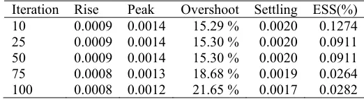
In Table 10, we see that we have 4 difference sets of PID parameters, therefore we will get 4 difference outputs. By using the value of PID parameters in Table 10, the output system can be seen in Fig. 15 and at Table 11.

Table 11: Output System with PID from Genetic Algorithm Using ISE Iteration Rise Peak Overshoot Settling ESS(%) 10 0.0009 0.0014 15.29 % 0.0020 0.1274 25 0.0009 0.0014 15.30 % 0.0020 0.0911 50 0.0009 0.0014 15.30 % 0.0020 0.0911 75 0.0008 0.0013 18.68 % 0.0019 0.0264 100 0.0008 0.0012 21.65 % 0.0017 0.0282

From Table 11, we can say that the rise time, peak time, and settling time become faster for later generation. The error steady state showing a pretty decent difference between 10th _{generation and 100}th

generation. But, the overshoot has a reverse effect. It became worse for the later generation.

For comparing the result, we’ll only use the best from each Index performance, that means the 100th

generation of each Index performance will be used for comparing the output.

Figure 15: Output System with PID Genetic Algorithm Using ISE

6. COMPARISON BETWEEN Z-N METHOD

AND GA

6.1.Comparison of The System

By using the value of the controllers that obtained earlier by using Z-N method and by GA, the output system by using that controller will be compared. PID parameters in 100th _{generation for each type of}

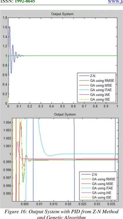
fitness value are used in the comparison. Output system using each controller is shown in Fig. 16.

Table 12: Output System with PID from Z-N Method and Genetic Algorithm

5067 Figure 16: Output System with PID from Z-N Method

and Genetic Algorithm

In Fig. 16, we can see that systems that using PID controller obtained by using GA are faster to go to the set point and going stable faster than controller that obtained by using Z-N method. For more information, the comparison between these methods can be found in Table 12.

For the rise time, from 0% to 90% of the set point, RMSE, MSE, and ISE have the same best time, 0.0008 second, so does the peak time, best peak time is obtained by using RMSE, MSE, and ISE in 0.0012 second. By using IAE, the system is producing the lowest overshoot, only 0.16% from the desired output. For the settling time, with error 5% from set point, IAE take the best time, in 0.0014 second. For error steady state, the system that using Z-N method, has the smallest error value, at 0.000000000000199% of the error.

Beside of that, the time needed to get the value of PID using GA, is around 0.5 seconds, for each generation. Therefore, for 100th _{generation, time}

needed is around 50 seconds, which is pretty slow compared to using SISO Tools to getting parameters from PID using Z-N Methods. But if we use 10th

generations which only need around 5 seconds to be generated, and compare them, we might get a faster system that make the output goes faster to its setpoints. This trial can be used for the industrial need, depend on what they need. If they need a faster system, and not too long to generated, Genetic Algorithm may satisfy its need.

6.2.Comparison Toward Constant Disturbance

After we got the value of controller PID, the next step is adding disturbance to the system plant, for constant disturbance the plant will be changed like in Fig. 17.

Figure 17: Plant System with Constant Disturbance

The result of the comparison between those two controllers on constant disturbance can be seen in Fig. 18.

5068 When we add a disturbance to second 0.5, with the value of disturbance is -1, we can see that the controller PID that obtained by using Z-N method shows the biggest oscillation. The rest of the controller have small effect, and still inside the 5% error of the set point. As we see in Fig. 18 and 19, the systems using PID from GA are more stable towards constant disturbance. GA with PID from IAE is the most stable of them, followed by MSE that is almost same with ISE and RMSE, and last is ITAE.

Figure 19: Output System with Constant Disturbance

6.3.Comparison Toward Random Disturbance

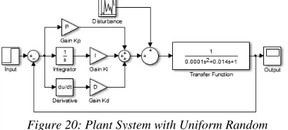
Next, we will compare those controllers by adding random disturbances. The system plant will be changed by adding uniform random number. We can see the system plant in Fig. 20. The value of the random disturbances varies from -1 to 1, for every 0.1 second.

Figure 20: Plant System with Uniform Random Disturbance

The result of this comparison can be seen in Fig 21. In Fig 21 we can see that both controller can maintenance the system to still at its set point, although the controller PID that obtained by using Z-N method have big oscillation. This oscillation will make the fin unstable and will waste more energy. As we zoom in the result, we’ll see that the systems using PID from GA are far more robust towards random disturbance. With the best of all is IAE and

then MSE, followed by ISE, then RMSE, and the last still ITAE.

Figure 21: Output System with Uniform Random Disturbance

7. CONCLUSIONS

From the analysis that we get above, we can conclude some of conclusions such as:

5069 2. The comparison between controllers shows that

PID controller from GA are faster to get the system to its set point than PID controller that obtained by using Z-N method, but have a bigger error steady state value.

3. With constant disturbance, all the controllers can maintenance the system to stay around the set point, although the controller that obtained by using Z-N method has a big oscillation.

4. For random disturbance in every 0.1 second, all the controller can maintenance the system to stay around the set point, although the controller that obtained by using Z-N method shows a big oscillation.

REFRENCES:

[1] Gauri, M. and N. R. Kulkarni, “Design and Optimization of PID Controller Using Genetic Algorithm”, IJRET: International Journal of Research in Engineering and Technology. Volume: 02 Issue:06 | Jun-2013. e-ISSN: 2319-1163 | p-ISSN: 2321-7308.

[2] Z. Supeng, F. Wenxing, Y. Jun and L. Jianjun, "Applying Genetic Algorithm to Optimization Parameters of Missile Control System", 2009 Ninth International Conference on Hybrid

Intelligent Systems, Shenyang, 2009, pp.

416-419.

[3] Mirzal, A., Yoshii, S., and Furukawa, M., “PID Parameters Optimization by Using Genetic Algorithm", STECS Journal, 2006, Vol. 8, pp. 34-43.

[4] M. L. Shahab, D. B. Utomo, and M. I. Irawan, “Decomposing and Solving Capacitated Vehicle Routing Problem (CVRP) Using Two-Step Genetic Algorithm (TSGA),” JATIT, vol. 87, no. 3, pp 461 – 468.

[5] Hozairi, Ketut Buda A., Masroeri, and M. I. Irawan, “Implementation of Nondominated Sorting Genetic Algorithm – II (NSGA–II) for Multiobjective Optimization Problems on Distibution of Indonesian Navy Warship”, JATIT, vol 64, no. 1, pp 274 – 281.

[6] Philip Hays, 2009, “Gunner’s Mate 3 & 2,” USA: Government Printing Office.

[7] Harris C.M., Piersol, A.G., 2002, “Harris' Shock and Vibration Handbook (5th _edition)”,

McGraw-Hill, ISBN 0-07-137081-1.

[8] Scott J. Moody. 1988. “Missile Actuator

Simulator and an Investigation into The Accuracy of Range-Kutta Numerical Integration,” Alabama: U.S. Army Missile Command.

[9] Entin Martina Kusumaningtyas. “Diktat Kecerdasan Buatan,” unpublished.