INTERACTION FORCES-RANDOM WALK MODEL
IN TRADITIONAL PATTERN GENERATION
PURBA DARU KUSUMA
School of Electrical Engineering, Telkom University, Bandung, Indonesia
E-mail: [email protected]
ABSTRACT
There are many traditional decorative patterns in Indonesia. Some of them are regular pattern. The advantage of regular one is its simplicity and easiness to be built by iterative algorithm. The disadvantage is it is monotonous. So, stochastic method can be implemented into regular pattern to add uncertainty. In this paper, the uncertainty was added by implementing combination of deterministic and stochastic approach into the regular pattern. The deterministic part is represented by modified interaction forces method. The stochastic part is represented by random walk method. This model also implemented multi agent approach by using two types of agent: starting point determinant and walker. In this paper, walker still walks until it cannot walk anymore. There are two parameters that are tested, the travelled nodes and the occupied cells ratio. In this research, by using interaction force as movement model, the occupied cell ratio is above 50 percents.
Keywords: Pattern Generation, Interaction Forces, Multi Agent, Random Walk, Batik
1. INTRODUCTION
Indonesia is a country that is rich with traditional heritage. One of the evidences is there are many traditional art patterns. These patterns can be found in the traditional building, wall, painting, paper, and fabric. The most popular pattern is Batik. There are many patterns that can be found in Batik, such as: Sidomukti, Sidomulyo, Liong, Rangrang, etc. As conservation effort, improvisations have been done in many ways to modernize these patterns.
One useful tool to modify traditional pattern is computation technique. Some studies in computer science have been done to explore Batik pattern [1-7]. Rangkuti has studied batik pattern classification based on the content of the pattern [4,5] and one of them used wavelet transform and fuzzy neural network [5]. The other studies have made modification by extracting geometric features of the original patterns and then made some modifications in geometric features position [2] or in pattern complexity [3].
Kusuma has made modification in traditional regular pattern based on cellular automata model [6,7]. One of them implemented pedestrian dynamic method [7]. These studies explored regular pattern because of its simplicity so
it can be easier to be made by computer program [6,7]. The modifications have been done by adding some uncertainties to enrich the regular pattern [6,7]. One of them implemented fully stochastic method [6] and the other implemented combination between stochastic and deterministic method [7]. All of them are built based on cellular automata model, fix iteration, and multi agent system. The problem in the previous works is by using the small number of agents, the occupied cell ratio was still below 50 percents. It is because the agents cannot move anymore before the iteration stops [6,7]. So, increasing the number of occupied cells ratio to above 50 percents with same number of agents by extending travelling distance is still challenging.
In this paper, the new model is proposed to improve the occupied cell ratio problem. This model is developed by combining the modified interaction force and random walk. Interaction force method acts as collision avoidance part. In its origin, interaction force is a part of social forces model that is used to avoid collision between persons [8-12].
Random walk is used in climbing plants competing for space [19], root growth and maneuver [20-22], and many more. These researches used directed random walk because the pattern is not full random because of some factors, such as gravity [20-22] or other plants [19].
This model uses discrete approach. Basically, interaction force is continuous. So, the interaction force calculation is simplified and transformed into discrete form. This model consists of two steps. The first step is determining the agents’ starting point position. In this step, this research implements two methods: random walk and uniform distribution. The second step is the agent’s movement. In this step, this research implements three methods: random walk, interaction force, and combination of interaction force and random walk.
The organization of the rest of this paper is as follows. Section 2 describes the previous works in interaction force. Section 3 explains the proposed model. Section 4 explains the implementation and result analysis. Section 5 concludes the work and describes the future research potentials.
2. INTERACTION FORCE
Interaction force is one of forces in social forces model [8]. This force occurs by the interaction between persons [8]. This model has been implemented and modified in pedestrian movement models. Basically, this model is continuous and deterministic [8]. Some researches converted this model into discrete platform, such as cellular automata, to simplify the calculation [9-11]. Some researches modified the basic social forces model by adding another forces so the modified model is suit for specific purposes [9-12].
Interaction force has similar function with repulsive force, which its function is avoiding person from collision [12]. When person moves, they may meet other persons or obstacles. As collision avoidance part, interaction forces has similar function with gyroscopic forces [13,14]. There is difference between interaction force and gyroscopic force. Interaction force makes person move away from the obstacle. Gyroscopic force makes person encircle the obstacle.
Detection shell is introduced in social forces model as observation area for each moving agent [13,14]. Agent only detects obstacle in his
detection shell [13,14]. Agent will not detect obstacle outer his detection shell.
3. PROPOSED MODEL
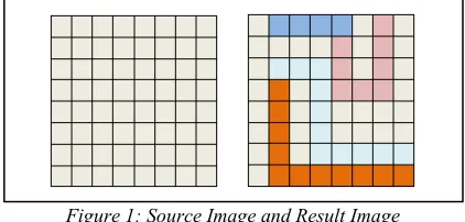
[image:2.612.312.523.361.462.2]Two dimensions image can be presented as a two dimensions matrix. In this representation, each cell represents the image pixel. The lowest index is in the left-top position. In a regular pattern, there is only one pattern object. One cell represents one object and one object may consist of more than one pixel. It can be said that the value of each cell is same and it can be valued as 0. In this research, this image will be manipulated so that there are cells with their value are not 0 and it is done randomly. The input of the system is the regular pattern image and the output of the system is the manipulated pattern image. It is illustrated in Figure 1. The left image represents the source image where the all cells value is 0. The right image represents the result image where there are some cells with their value is not 0.
Figure 1: Source Image and Result Image
In this model, there are agents that the role is change the value of the cells they passed by the value of the agents. For example, there are three agents which their value are 1,2, and 3 consecutively. Each agent walks randomly. During the iteration, each agent will move from one cell to another cell. The agent can move to the cell only if the cell value is 0 which means that the cell has never been passed by other agent. The agent still moves until it cannot find available cell in its neighbor. The iteration will stop only if there is not any agents can move anymore. It is different with the previous works where the iteration is set statically [1][2]. Figure 2 describes the main process algorithm. Variable n represents the number of agents. Variable m represents the number of agents that can walk. Variable pi is the position of
agent i. setstartposition is a function to determine the starting position of the agent. walk() is procedure that makes the agent walks. checkpossibilitywalk() is function that is used to calculate the number of agents that still can walk.
Figure 2: Main Process Algorithm
The main process contains two processes. The first process is the starting point determination of each agent. The second process is the movement iteration. The first process is executed by agent named starting point determinant. The second process is executed by agent named walker.
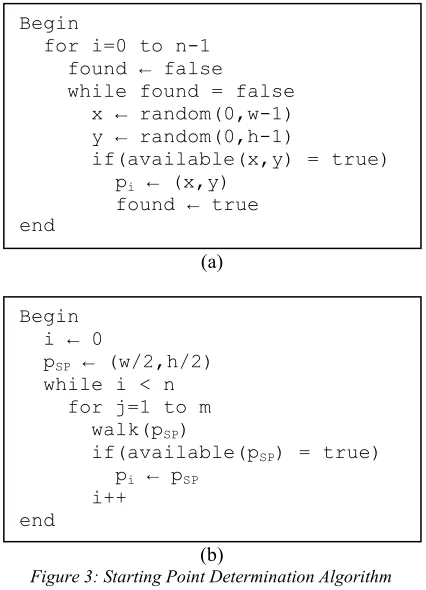
There are two stochastic methods that are used to determine the starting point. The first method is by using uniform distribution. The second method is by using random walk. The performance of these methods then will be compared to each other. In the first method, the x position is determined randomly between 0 to matrix width and y position is determined randomly between 0 to matrix height. If there is other agent that has occupied this cell, the process is repeated. This process is iterated until all walkers’ starting point is determined. The process of the second method is described as follows. The starting point agent starts from the center of the image matrix. The starting point agent walks randomly with four possible directions (up, right, down, left). After m steps, the starting point determinant checks the availability of the cell. If the cell is available, this cell will be allocated for the walker. This process still iterates until all walkers have starting point. These algorithm processes are illustrated in Figure 3. Part a is for uniform distribution based method and part b is for random walk based method.
The next process is movement method. In this research, there is only one kind of force in social forces model, which is interaction force that is used in the movement method. The motivation of ignoring other forces such as desired movement force and attracting force is preventing collision or path cross with other agents. In this research, there are three methods: fully random walk, fully interaction force, and combination of random walk and interaction force. In the first method, the movement is fully stochastic. In second method, the movement is fully deterministic. In the third method, the movement is combination of stochastic and deterministic. In random walk method, The
walker i’s position at time t can be symbolized with pi(t). This position is determined by the walker’s
previous position and the independent and identically distributed (iid) random variable which is symbolized with Xi,t. Equation (1) describes this
formula. Xi,t contains two value that represents x
and y coordinates. The neighbor cells of walker i’s current position is represented with set A that contain {a1,a2,a3,a4}. The relation of variable a and
the walker i’s position is described in Table 1. The value of each variable a is determined based on the availability of the cell. If the cell is available, so the value of variable a is 1 and otherwise is 0. The availability of the grid is represented by s(x,y) which is the status of the cell at x and y position. This is described in Equation (2). The probability of each variable a is described in Equation (3). In Equation (3), it can be seen that if the cell is unavailable then the probability of walker will move to that cell is 0. The probability of a walker move to an available cell among all walkers available neighbor grid is equal.
(a)
(b)
Figure 3: Starting Point Determination Algorithm
X
p
p
i,t=
i,t−1+
i,t (1)
=
=
=
0
)
(
,
1
1
)
(
,
0
a
a
a
b b
b
s
s
(2)
Begin i ← 0
pSP ← (w/2,h/2)
while i < n for j=1 to m
walk(pSP)
if(available(pSP) = true)
pi ← pSP
i++ end
Begin
for i=0 to n-1 found ← false
while found = false x ← random(0,w-1) y ← random(0,h-1)
if(available(x,y) = true)
pi ← (x,y)
found ← true end
begin for i = 0 to n-1
pi ← setstartposition()
m ← n
while m ≠ 0
for i = 0 to n-1 walk(i)
[image:3.612.312.525.357.652.2]∑
=
a
P
a
a
bb
)
[image:4.612.306.517.52.655.2](
(3)Table 1: The Relationship Between Variable a and Walker’s Position
Walker i’s neighbor
Relative position
ω(ab)
(degree) a1 ax = px-1 ;
ay = py
270
a2 ax = px ;
ay = py-1
180
a3 ax = px+1 ;
ay = py
0
a4 ax = px ;
ay = py+1
90
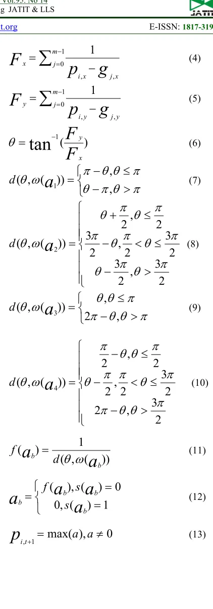
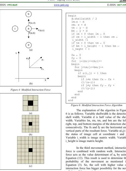
In interaction force method, the walker’s position at time t is determined by the interaction force resultant around the walker. Detection shell is implemented to identify any unavailable cells. Illustration of interaction force can be seen in Figure 4. Detection shell is an observation area around the agent. Agent detects only grids inside its detection shell. When the detection shell is wider, the number of grids that must be calculated is increased. The motivation of the detection shell is that wider detection shell will improve the agent’s collision avoidance capability. In the other hand, wider detection shell makes the computation heavier. In this research, the detection shell is square with d is the side size. Agent’s position is in the center of the detection shell. Figure 5 illustrates the detection shell. The resultant force is symbolized with Fr with Fx is the horizontal part
and Fy is the vertical part. The value of Fx and Fy
are calculated by using Equation (4) and (5). Variable m is number of unavailable grids in the detection shell. j is index for unavailable grid in detection shell. θ is angle between Fy and Fx. ω(ab)
is the absolute angle of ab. d(θ,ω(ab)) is the angle
difference between θ and ω(ab) and is calculated by
using Equation (7), (8), (9), or (10). By using Equation (11), the value of f(ab) is inversely
proportional with the angle distance between θ with ω(ab). Finally the value of ab is determined by the
availability of that grid. If the grid is unavailable, the value of ab is 0. Otherwise, it calculated by the
value of f(ab).
∑
− =−
=
1 0 , ,1
m j x j x i xg
p
F
(4)
∑
− =−
=
1 0 , ,1
m j y j y i yg
p
F
(5)
)
(
tan
1F
F
x y −=
θ
(6)
>
−
≤
−
=
π
θ
π
θ
π
θ
θ
π
ω
θ
,
,
))
(
,
(
1a
d
(7)
>
−
≤
<
−
≤
+
=
2
3
,
2
3
2
3
2
,
2
3
2
,
2
))
(
,
(
2π
θ
π
θ
π
θ
π
θ
π
π
θ
π
θ
ω
θ
a
d
(8)
>
−
≤
=
π
θ
θ
π
π
θ
θ
ω
θ
,
2
,
))
(
,
(
3a
d
(9)
>
−
≤
<
−
≤
−
=
2
3
,
2
2
3
2
,
2
2
,
2
))
(
,
(
4π
θ
θ
π
π
θ
π
π
θ
π
θ
θ
π
ω
θ
a
d
(10)))
(
,
(
1
)
(
a
a
b bd
f
ω
θ
=
(11)
=
=
=
1
)
(
,
0
0
)
(
),
(
a
a
a
a
b b b bs
s
f
(12)0
),
max(
1 ,≠
=
+
a
a
Figure 4: Modified Interaction Force
Figure 5: Detection Shell
Based on the concept that is described in Equation 4 and Equation 5 and illustration in Figure 4 and Figure 5, the algorithm to determine Fx and
Fy can be developed. Parameters that are involved
are shell size, image matrix size, and the cell value. The algorithm is described in Figure 6.
Figure 6: Modified Interaction Force Algorithm
The explanation of the algoritm in Figure 6 is as follows. Variable shellwidth is the detection shell width. Variable d is half value of the shell width. Variables lm, rm, tm, and bm are the left, right, top, and bottom margins of the detection shell consecutively. The fx and fy are the horizontal and vertical parts of the resultant force. Variable s(i,j) is the status of image cell at coordinate i and j. Variable i_width is image matrix width. Variable i_height is image matrix height.
In the third movement method, interaction force is combined with random walk. Interaction force acts as the value determinant of ab by using
Equation (12). This result is used to determine the probability of the movement as mentioned in Equation (3). So, the cell with higher value of interaction force has bigger possibility for the next cell that will be occupied.
4. IMPLEMENTATION AND RESULT
DISCUSSION
The proposed models are implemented into the application that generates Tenun based pattern objects. The image consists of 50 cells (a)
(b)
(a)
(b)
(c)
begin
d←shellwidth / 2 lm←x – d
rm← x + d tm ← y – d bm ← y + d
if lm < 0 then lm ← 0
if rm > i_width – 1 then rm ← i_width -1
if tm < 0 then tm ← 0
if bm > i_height – 1 then bm ← i_heght + 1
fx ← 0 fy ← 0
for i=lm;i<=rm;i++ begin
for j=tm;j<=bm;j++ begin
if s(i,j) = 1 then begin
if i≠x then fx ← fx + (1/(x-i))
if j≠y then fy ← fy + (1/(y-j))
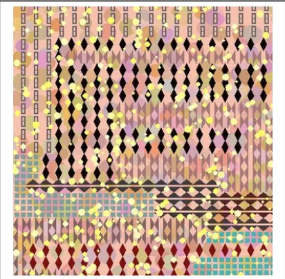
width and 25 cells height. The cell dimension is 20 x 20 pixels. The result image can be seen in Figure 7. In Figure 7, the pattern is looked random too. The number of walkers is 10.
Figure 7: Result Image
[image:6.612.316.522.186.400.2]This basic image can be improved in many ways. First improvization is by adding the backgroud and foreground pattern in the image. The example of this improvization is illustrated in Figure 8. In this image, the background and foreground pattern is circle objects that are placed randomly. The random method in placing the position of the circles follows uniform distribution. The circles in the background are bigger than circles in the foreground. The color of the background circles is randomized too. Meanwhile, the color of the foreground circles is same to each other.
Figure 8: First Modification Image
The improvization can also be done in the pattern objects. The object can be Batik object. Batik object is identical with dot or small circle
object. The set of circle can form new object, such as flower, leaf, or animal. The example of this improvization is illustrated in Figure 9. In Figure 9, there are four objects. The first is flower object that is arranged by four oval objects. The second is a big circle that is surrounded by four small circles. The third is big circle that consists of five small circles. The fourth is matrix of four small circles.
Figure 9: Second Modification Image
Based on the proposed model and compared with the existing model. In the existing model which is also creating traditional pattern using social forces model, there is destination point so the walker’s goal is reaching the destination [7]. In this research, the walker does not use the destination point. In the existing model, there are four neighbor cells that are used in the calculation [6,7]. In this research, there are more than four neighbor cells that are used in the calculation and it is depended on detection shell. Because the proposed model is developed based on discrete approach, the agent’s directions is limited into four options. This is different with the basic social forces model that uses continuous approach [8]. This proposed model use one kind of force only from the basic social forces model. The attracting force, repulsive force, and desired movement force are ignored [8].
[image:6.612.91.297.460.661.2]between starting point position and the center of the image matrix. The second is the correlation between the starting point method and the occupied cells ratio. The observed parameter in movement testing is occupied cells ratio.
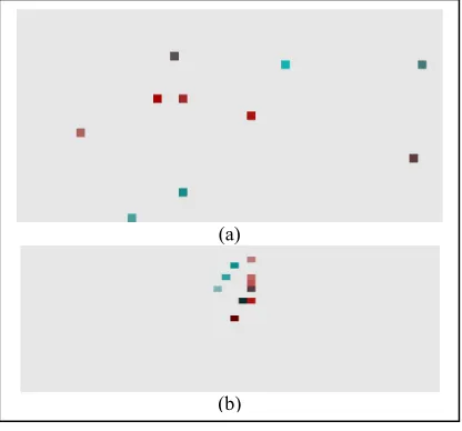
[image:7.612.317.523.88.140.2]There are two methods that are compared to each other in starting point determination, the uniform distribution and random walk. In random walk based, the number of steps (m) is from 5 steps to 50 steps with the gap is five. There are 30 sessions for every test. Figure 10 illustrates the result image. Figure 10a illustrates the starting point distribution based on uniform distribution. Figure 10b illustrates the starting point distribution based on random walk. It can be seen that when it is generated by using random walk, the starting point distribution is more clustered.
Figure 10: Starting Point Distribution
The quantitative result of average distance of the starting point that is generated by using uniform distribution is as follows. By using uniform distribution, the average distance for 30 testing sessions is 14.69. The minimum average distance is 9.57. The maximum average distance is 18.96. The result of the average distance of random walk based starting point is in Table 2. There are 30 testing sessions for every value of m.
Table 2: Average Distance Using Random Walk
m Average Distance
Average Minimum Maximum 5 4.92 2.10 11.35 10 7.27 3.17 14.38 15 7.99 3.29 20.08 20 8.32 3.89 15.00 25 8.71 4.24 17.72 30 8.86 5.24 15.70
35 9.93 4.85 19.25 40 9.99 5.43 18.59 45 10.46 5.25 14.39 50 10.41 6.77 16.47
The next testing group is movement test. There are three movement models: random walk, interaction force, and combination between interaction force and random walk. There are two starting point determination model for each movement model: uniform distribution and random walk. There are 30 test sessions when it used uniform distribution as starting point determination model and there are 30 test sessions too for every number of steps when it used random walk one.
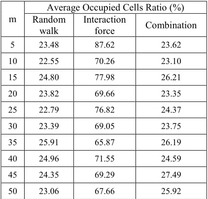
First movement model test is random walk based movement test. When the starting point determination is using uniform distribution, the average occupied cells ratio is 33.58 percents. The minimum occupied cells ratio is 25.36 percents. The maximum occupied cells ratio is 46.16 percents. The occupied cell ratio result when using random walk for starting point determination is in Table 3 column 2. There are 30 testing sessions for every value of m. Based on data in Table 3 column 2, we can see that the number of steps doesn’t affect the occupied cells ratio. The minimum occupied cells ratio is 22.55 percents. The average occupied cell ratio is 23.91 percents. The maximum occupied cell ratio 25.91. So, the occupied cell ratio is still below 40 percents. In occupied cells ratio, the uniform distribution based starting point determination model is better than random walk based one.
Second movement model test is interaction force based movement model. In this test, the side size of the detection shell is 5. When the starting point determination model is using uniform distribution, the result is as follows. The average occupied cells ratio is 69.14 percents. The minimum occupied cells ratio is 40.4 percents. The maximum occupied cells ratio is 93.12 percents. When using random walk model for starting point determination, the result is in Table 3 column 3 and it can be seen that the number of steps doesn’t affect the occupied cells ratio. The average occupied cells ratio is 72.58 percents. The minimum cell ratio is 65.87 percents. The maximum occupied cell ratio is 87.62. Comparing the starting point determination model, the random walk based model is better than the uniform distribution based one.
The third movement model test is interaction force-random walk combination model. (a)
[image:7.612.91.299.296.490.2]The side size of the detection shell is 5. When the starting point determination model is using uniform distribution, the result is as follows. The average occupied cells ratio is 30.88 percents. The minimum occupied cells ratio is 22.72 percents. The maximum occupied cells ratio is 43.12 percents. When starting point determination model is using random walk, the result is in Table 3 column 4. The average occupied cells ratio ranges from 24.85 percents. The minimum occupied cells ratio is 23.1 percents. The maximum cells ratio is 27.49 percents. The number of steps doesn’t affect the result. In this movement model, the uniform distribution based starting point determination model makes better result rather than random walk based one.
Table 3: Average Occupied Cell Ratio
m
Average Occupied Cells Ratio (%) Random
walk
Interaction
force Combination 5 23.48 87.62 23.62
10 22.55 70.26 23.10
15 24.80 77.98 26.21
20 23.82 69.66 23.35
25 22.79 76.82 24.37
30 23.39 69.05 23.75
35 25.91 65.87 26.19
40 24.96 71.55 24.59
45 24.35 69.29 27.49
50 23.06 67.66 25.92
Based on the explanation above, by using interaction force model as movement model, the average occupied cell ratio is higher than 50 percents even uniform distribution or random walk method are used to determine the starting point position but random walk model creates better occupied cell ratio rather than uniform distribution model. When using random walk or combination of random walk and interaction force model as movement model, the occupied cell ratio is still below 50 percents. When using uniform distribution model as starting point determination model, random walk model creates better average occupied cell ratio rather than combination of interaction force and random walk as movement model. When using random walk model as starting point determination model, combination of random walk and interaction force creates better average
occupied cell ratio rather than random walk as movement model. The using of interaction force model create better occupied cell ratio compared with the previous work [6][7]. When using simple cellular automata, the occupied cells ratio is 47.4 percents [6]. When using pedestrian dynamics, the occupied cells ratio is 42.3 percents [7].
5. CONCLUSION AND FUTURE WORK
Based on the explanation above, there are new methods that are proposed in this research. First, this proposed method uses only one kind of force rather than the basic social forces model that contains four kinds of forces. Second, the square detection shell has been used so that the number of neighbor cells that must be observed in the calculation is increasing. Basically, the shape of the detection force is circle.
The proposed models have been developed and have been implemented in modifying the regular traditional art pattern. The result image also can be improved. In this research, two improvizations are proposed. In the first improvization, foreground and background patterns is added to enrich the result image. In the second improvization, Batik objects that are identical with small circles or dots are used to change Tenun object. It has met the research goal which is increasing the number of occupied cells ratio. When using social forces model, the occupied cells ratio is above 50 percents so that the research goal is accomplished. When using full random walk or the combination between random walk and interaction force, the occupied cell ratio is below 50 percents. It is also become the other research finding in this paper. By removing the desired movement force which is the destination point and the movement become fully deterministic, the occupied ratio is high. It means that the existence of the stochastic part reduces the occupied ratio.
REFERENCES:
[1] A.E. Minarno, A. Kurniawardhani, F. Bimantoro, “Image Retrieval Based on Multi Structure Co-occurrence Descriptor”,
TELKOMNIKA, vol. 14(3), 2016, pp.1175-1182.
[2] A.E. Minarno, N. Suciati, “Batik Image Retrieval Based on Color Difference Histogram and Gray Level Co-Occurrence Matrix”, TELKOMNIKA, vol. 12(3), 2014, pp.597-604.
[3] A. Fanani, A. Yuniarti, N. Suciati, “Geometric Feature Extraction of Batik Image Using Cardinal Spline Curve Representation”,
TELKOMNIKA, vol.12(2), 2014, pp.397-404. [4] H.A. Rangkuti, A. Harjoko, A.E Putro,
“Content Based Batik Image Retrieval”,
Journal of Computer Science. 10(6), 2014, pp.925-934.
[5] A.H Rangkuti, “Content Based Batik Image Classification Using Wavelet Transform and Fuzzy Neural Network”, Journal of Computer Science, 10(4), 2014, pp.604-613.
[6] P.D Kusuma, “Traditional Fabrics Pattern Modification using Cellular Automata”,
Proceeding of National Conference on Information Technology Application, Yogyakarta, 2016, D1-5.
[7] P.D. Kusuma, “Implementation of Pedestrian Dynamics in Cellular Automata Based Pattern Generation”, International Journal of Advanced Computer Science and Applications (IJACSA), 7(3), 2016, pp.65-70.
[8] D. Helbing, P. Molnar, “Social Forces Model for Pedestrian Dynamics” Physical Review E, 51(5), 1995, pp.4282-4286.
[9] W. Song, Y.F. Yu, W.C. Fan, “A Cellular Automata Evacuation Model Considering Friction and Repulsion”, Science in China Series E-Engineering and Material Science, 48(4), 2005; pp.403-413.
[10] W. Song, X. Xu, B.H Wang, S. Ni, “Simulation of Evacuation Process Using a Multi Grid Model for Pedestrian Dynamics”,
Physica A, 363(2), 2006, pp.492-500.
[11] X. Ji, J. Zhang, Y. Hu, B. Ran, “Pedestrian Movement Analysis in Transfer Station Corridor: Velocity Based and Acceleration Based”, Physica A. vol.450, 2016, pp.416-434.
[12] T. Korecki, D. Palka, J. Was, “Adaptation of Social Force Model for Simulation of Downhill Skiing”, Journal of Computational Science, vol.16, 2016, pp.29-42.
[13] D.E. Chang, J.E. Marsden, “Gyroscopic Forces and Collision Aviodance with Convex Obstacles, New Trends in Nonlinear Dynamics and Control and Their Applications”, Lecture Notes in Control and Information Science, vol.295, 2004; pp.145-159.
[14] D.E. Chang, S.C Shadden, J.E Marsden, R. Olfati, “Collisison Avoidance for Multiple Agent Systems”, Proceeding of the 42nd IEEE Conference on Decision and Control, Hawaii, Dec. 2003.
[15] M. Szczpanski, B. Smolka, D. Slusarczyk, K.N. Plantaniotis, A.N. Venetsanopoulos, “Geodesic Paths Approach to Color Image Enhancement”, Electronic Notes in Theoretical Computer Science, vol.46, 2001, pp.146-160.
[16] M. Szczpanski, B. Smolka, K.N. Plantaniotis, A.N. Venetsanopoulos, “On the Distance Function Approach to Color Image Enhancement”, Discrete Applied Mathematics, vol.139, no.1, 2004, pp.282-305.
[17] S. Choi, B. Ham, K. Sohn, “Hole Filling with Random Walks using Occlusion Constraints in View Synthesis”, Proceeding on International Conference on Image Processing. Bangalore, India, 2011.
[18] L. Grady, “Random Walks for Image Segmentation”, IEEE Transactions on Pattern Analysis and Machine Intelligence, vol.28, no.11, 2006; pp.1768-1783.
[19] B. Benes, E.U. Millan, “Virtual Climbing Plants Competing for Space”, Proceedings of The Computer Animation, 2002.
[20] A. Klopper, “Roots Manoeuvre”, Nature Physics, vol.11, 2015.
[21] A. Johnson, C. Karlsonn, T.H, Iversen, D.K. Chapman, J. Braseth, “Plant Growth and random Walk – An Experiment for IML-2”,
Life Sciences Research in Space, Proceedings of the Fifth European Symposium, September 26, 1993.