Theoretical study of photoinduced superconductivity in 2 2 2 8+d Bi Sr CaCu O (Bi2212) with two band model

Journal of Chemical and Pharmaceutical Research

ISSN No: 0975-7384 CODEN(USA): JCPRC5

J. Chem. Pharm. Res., 2010, 2(5): 131-152

Theoretical study of photoinduced superconductivity in

δ

+

8 2 2

2

Sr

CaCu

O

i

B

_{(Bi2212) with two band model}

Anuj Nuwal*1, S. L. Kakani2 and M. L. Kalra1

1

Department of Physics, University College of Science, M. L. Sukhadia University, Udaipur, (Raj.), India

2

Institute of Technology and Management, Bhilwara(Raj.), India

___________________________________________________________________________

ABSTRACT

Dependences of the superconducting transition temperature (T ) on hole concentration in c

δ + 8 2 2

2Sr CaCu O

i

B (Bi-2212) cuprate have been calculated in a frame work of canonical two-band BCS model containing Fermi surfaces of p and d holes. The shift of the chemical potential

( )

µ

leads to the curve T_c

( )

n with a maximum. The dependences of _h T_c

( )

n for our _h system compared with available experimental data. Self –consistent equations for superconducting order parameter

( )

∆ are derived using Green's functions and equation of motion method. The enhancement of T is found due to doping. _c

Keywords: Green’s function; p and d holes; critical temperature; hole concentration.

P A C S : 74.20.-z, 74.20.Fg, 74.20.Mn, 74.25. Bt

___________________________________________________________________________

INTRODUCTION

It is of fundamental importance to explain the doping dependences of superconducting properties of photoinduced high-T cuprates. Doping dependences of the electronic chemical _c

potential

( )

µ

have been measured in Bi₂Sr₂CaCu₂O_8+δ (Bi-2212) [ 1 ].

There are number of data indicating participation of several bands in the high-T c superconducting mechanism. Two bands are found to intersect the Fermi level in Bi-2212. In Bi₂Sr₂CaCu₂O_8+δ , the BiO-plane bands seem to be coupled to the Cu-O plane band [ 8]. In [2,3,4,9-10], a model of two over lapping hole bands has been used to reproduce the T _c

dependences on the hole doping La_2−xSr_xCuO₄,YBa₂Cu₃O_7−x and Bi₂Sr₂CaCu₂O_8+δ.

The optical reflectivity and the absorption spectra for the Bi2Sr2Ca_n−1Cu_nO_x systems (n =

1,2,3) were measured at room temperature using c-axis oriented films [11]. In the reflectivity spectra, an increase of n enhanced a Drude-like reflection and shifted its plasma edge to the shorter wavelength region. In the absorption spectra, near-infrared absorption was enhanced with increasing n. These features reflected in the electronic structure and hence the superconductivity. In Bi-2212 system, the optical absorption spectra consisted of four discrete bands peaking at about 4.3, 3.7, 2.0-2.5 and 1.5-1.7 eV. The energies of characteristic peaks in Bi-compounds remain practically constant when Bi atoms are partially replaced by Pb and Ca by Y or Er atoms [12].

Recent experimental investigations on high-T cuprates systems, having compositions in the c semiconductor regime, have shown light-induced changes, which are indicative of photoinduced superconductivity [13-25]. Although many aspects of the phenomena of

high-c

T layered cuprates remain unexplained, the transition from the insulating and

antiferromagnetic phase to the metallic and superconducting phase is known to be correlated with the density of charge carriers in the CuO plane [22]. ₂

In some cases there is an increase of the critical temperature T with radiation doses [ 16-18 ]. _c

The interesting result is the growth of the absolute value of diamagnetic moment almost clearly with radiation doses which saturates beyond a certain state [ 16 ]. The onset of transient photo induced super-conductivity, at high excitation levels, is a real phenomenon [ 15, 19 ].

The transient photo-induced super-conductivity is persistent at low temperatures and relax within days at room temperature [16, 20 ].

In this paper, we consider the photoinduced effect in cuprates superconductors taking into account the canonical two band model with p and d holes. The photoinduced effect induces the changes of hole concentration and leads to the change in superconducting properties. First we shall calculate the superconducting order parameters both for p and d holes and then calculate the dependences of superconducting transition temperature

( )

T on hole _c

concentration

( )

n in _h Bi₂Sr₂CaCu₂O_8+δ (Bi-2212) . This model can easily be generalized to two band system.

2. The Model Hamiltonian

The pairing mechanism in photoinduced superconductor is presently a subject of a vivid debate. There is great suspicion that some, if not all, photoinduced compounds are unconventional.

comparable to the gap value for photoinduced cuprates which requires consideration of the band structure, chemical potential and superconducting on an equal footing. This problem needs careful experimental and theoretical investigation.

The Mechanism of photoinduced superconductivity has been extensively studied but photoinduced superconductivity in cuprates is still to be being understood theoretically. One of the approaches for the photoinduced superconductivity in cuprates, at present lies in the two component scenario [4, 26, 27-30].

Our two-band model, in the context of photoinduced superconductivity, has common features with other models [4, 26].

In this paper, we present the self consistent calculations of the dependences of the chemical potential

( )

µ

and the superconducting transition temperature

( )

T on the hole c concentration

( )

n in the h Bi2Sr2CaCu2O8+δ system.

We consider the following Hamiltonian for photoinduced two band structure [5] -

pd d

p

H H

H

H = ₀ + ₀ + ( 1 )

Where

(

)

∑

∑

∑

∈ + + ₋+ ₋ +∆+ ₋ +∆ + +−

=

p

p p

pp p

p p pp p

p p p

p p p

C C C

C C

C C C

H_{0 σ σ σ' σ' σ σ'} σ σ' ( 2 )

(

)

∑

∑

∑

∈ + + ₋+ ₋ +∆+ ₋ +∆ + +−

=

d

d d

dd d

d d dd d

d d d

d d d

C C C

C C

C C C

H_{0 σ σ σ' σ' σ' σ} σ σ' ( 3 )

and

∑

∑

∑

∑

− + + −

− −

+ +

− + + −

− −

+ +

+ +

+ =

d

d d

p p pd p

p p d

d pd

p

p p

d d

pd d

d d p

p pd pd

C C C

C V C C C

C V

C C C

C V C C C

C V H

' '

' '

' '

' '

σ σ

σ σ σ

σ σ

σ

σ σ

σ σ

σ σ σ

σ

( 4 )

Where p and d are momentum labels in the p and d bands respectively with energies ∈_p and d

∈ , µ is the common chemical potential. Each band has its proper pairing interaction V_pp

and V_dd, while the pair interchange between the two bands is assured by V_pd term.

We have assumedV_pd =V_dp, and we define the following quantities:

µ

µ

∈ =∈ −

− =∈

∈ 0 0

d d p

p

' σ

σ p

p pp

pp V C C −

+ + + ₌

∆

' σ

σ d

d dd

dd V C C −

+ + + ₌

∆

Further we define –

' 1 Vpd Cpσ C −pσ

+ + + ₌

∆

' 2 Vpd Cdσ C −dσ

+ + + ₌

Now H_pd in equation ( 1 ) reads as

∑

∑

∑

∑

₋ +− + + ₋ + +− + _{+∆ +∆ +∆} ∆ = d d d p p p p p p d d d

pd C C C C C C C C

H _{1 σ' σ 2} σ' σ _{2 σ' σ 1 σ} σ'

So final Hamiltonian can be written as

(

)

(

)

∑

∑

∑

∑

∑

∑

∑

∑

∑

∑

− + + − + + − + − + − + + − + − + − + − + + − + − + − + ∆ + ∆ + ∆ + ∆ + ∆ + ∆ + + ∈ + ∆ + ∆ + + ∈ = d d d p p p p p p d d d d d d dd d d d dd d d d d d d p p p pp p p p pp p p p p p p C C C C C C C C C C C C C C C C C C C C C C C C H ' 1 ' 2 ' 2 ' 1 ' ' ' ' ' ' ' ' σ σ σ σ σ σ σ σ σ σ σ σ σ σ σ σ σ σ σ σ σ σ σ σ

( 6 )

We study the Hamiltonian ( 6 ) with the Green’s function technique and following the equation of motion method .

2.1 GREEN’S FUNCTIONS

In order to study the physical properties, we define the following normal and anomalous Green’s functions [ 31-40 ] :

( a ) G_p

(

p,τ −τ'

)

=− T_τ C_pσ(τ)C+pσ(τ') ( b ) G_d

(

d,τ −τ'

)

=− T_τ C_dσ(τ)C+dσ(τ') ( c ) fp

(

p,τ−τ'

)

= Tτ C−pσ'(τ)Cpσ(τ') ( d ) fd

(

d,

τ

−

τ

'

)

= Tτ C−dσ'(

τ

)Cdσ(

τ

') ( e ) f_p+

(

p,τ −τ'

)

= T_τ C+pσ(τ)C+−pσ'(τ')

( f ) f_d+

(

d,τ −τ'

)

= T_τ C+dσ(τ)C+−dσ'(τ') ( 7 )

These Green’s functions satisfy the following equations:

(

ω

−

∈

_p

)

〈〈

C

_pσ

,

C

+pσ

〉〉

=

δ

_pp'

−

(

∆

_pp

+

∆

₂

)

〈〈

C

+pσ

,

C

+−pσ'

〉〉

( 8 )

(

ω

₋

_∈

_d

)

〈〈

C

_dσ

,

C

+dσ

〉〉

₌

δ

_dd'

₋

(

_∆

_dd

₊

_∆

₁

)

〈〈

C

+dσ

,

C

+−dσ'

〉〉

( 9 )

(

₋

_∈

)

〈〈

〉〉

₌

₋

(

_∆

₊

_∆

)

〈〈

+

〉〉

− σ σ σ σ

ω

p

C

p '

,

C

p pp 2

C

p

,

C

p ( 10 )

(

−

∈

)

〈〈

〉〉

=

−

(

∆

+

∆

)

〈〈

+

〉〉

− σ σ σ σ

ω

d

C

d '

,

C

d dd 1

C

d

,

C

d ( 11 )

(

+

∈

)

〈〈

〉〉

=

−

(

∆

+

+

∆

+

)

〈〈

+

〉〉

− + + σ σ σ σ

ω

_p

C

p

,

C

p ' pp ₂

C

_p

,

C

p ( 12 )

(

+

∈

)

〈〈

〉〉

=

−

(

∆

+

+

∆

+

)

〈〈

+

〉〉

− + + σ σ σ σ

ω

_d

C

d

,

C

d ' dd ₁

C

_d

,

C

d ( 13 )

Further, we also obtain

(

+

∈

)

〈〈

+

〉〉

=

−

(

∆

+

+

∆

+

)

〈〈

₋

〉〉

σ σ σ

σ

δ

ω

p

C

p

,

C

p pp' pp 2

C

p '

,

C

p ( 14 )

(

+

∈

)

〈〈

+

〉〉

=

−

(

∆

+

+

∆

+

)

〈〈

₋

〉〉

σ σ σ

σ

δ

ω

d

C

d

,

C

d dd' dd 1

C

d '

,

C

d ( 15 )

(

∆

pp

+

∆

2

)

=

∆

p and

∆

p

≅

∆

p +

(

∆dd +∆1

)

=∆d and

∆

d

≅

∆

d

+

Then

(

∆

+pp

+

∆

+2

)

=

∆

+p

≅

∆

_p

(

∆

+dd

+

∆

+1

)

=

∆

+d

≅

∆

_d ( 16 )

One can rewrite the equations ( 8 ) to ( 15 ) using (16 ) as ,

(

ω

₋

_∈

_p

)

〈〈

C

_pσ

,

C

+pσ

〉〉

₌

δ

_pp'

₋

_∆

_p

〈〈

C

+pσ

,

C

+−pσ'

〉〉

( 17 )

(

ω

−

∈

_d

)

〈〈

C

_dσ

,

C

+dσ

〉〉

=

δ

_dd'

−

∆

_d

〈〈

C

+dσ

,

C

+−dσ'

〉〉

( 18 )

(

ω

₋

_∈

_p

)

〈〈

C

_−pσ'

,

C

_pσ

〉〉

₌

₋

_∆

_p

〈〈

C

+pσ

,

C

_pσ

〉〉

( 19 )

(

−

∈

)

〈〈

〉〉

=

−

∆

〈〈

+

〉〉

− σ σ σ σ

ω

d

C

d '

,

C

d d

C

d

,

C

d ( 20 )

(

₊

_∈

)

〈〈

〉〉

₌

₋

_∆

〈〈

+

〉〉

− + +

σ σ

σ σ

ω

_p

C

p

,

C

p ' _p

C

_p

,

C

p ( 21 )

(

+

∈

)

〈〈

〉〉

=

−

∆

〈〈

+

〉〉

− + +

σ σ

σ σ

ω

_d

C

d

,

C

d ' _d

C

_d

,

C

d ( 22 )

(

₊

_∈

)

〈〈

+

〉〉

₌

₋

_∆

〈〈

₋

〉〉

σ σ σ

σ

δ

ω

p

C

p

,

C

p pp' p

C

p '

,

C

p ( 23 )

(

+

∈

)

〈〈

+

〉〉

=

−

∆

〈〈

₋

〉〉

σ σ σ

σ

δ

ω

d

C

d

,

C

d dd' d

C

d '

,

C

d ( 24 )

Finally, one obtains the Green’s functions by solving coupled equations ( 17 ) to ( 24 ) as : ( a ) Green’s function for p-holes :

>>

<<

+

− +

'

,

_σ

σ _p

p

C

C

=

(

2 2

)

p p

E

−

∆

−

ω

( 25 )

>>

<<

+

σ

σ p

p

C

C

,

=

(

(

2 2

)

)

p p

E

−

∈

−

ω

ω

( 26 )

(

)

(

E

P

)

C

C

_p

,

_{p 2} p₂

−

∈

+

=

>>

<<

+

ω

ω

σ

σ ( 27 )

( b ) Green’s function for d-holes :

>>

<<

+

− +

'

,

_σ

σ _d

d

C

C

=

(

2 2

)

d d

E

−

∆

−

ω

( 28 )

>>

<<

+

σ

σ _d

d

C

C

,

=

(

(

2 2

)

)

d d

E

−

∈

−

ω

ω

( 29 )

>>

<<

+

σ

σ d

d

C

C

,

=

(

(

2 2

)

)

d d

E

−

∈

+

ω

ω

2.2 THE CORRELATION FUNCTIONS

Using the following relation [ 35-39 ] ,

ω

ω

π

ω βω ω

i

t

t

d

e

t

B

t

A

t

B

t

A

i

Limit

t

A

t

B

i i

_exp(

₍

_'

₎₎

1

)

'

(

;

)

'

(

)

'

(

;

)

'

(

2

)

(

)

'

(

0

+

×

−

−

〉〉

〈〈

−

〉〉

〈〈

=

〉

〈

_∫

+∞

∞ −

∈ + ∈

− ∈→

( 31 ) and employing the following identity ,

(

K

)

K

K

E

i

E

i

E

i

Limit

_

=

−











−

∈

−

−

−

∈

+

∈→

ω

ω

2

π

δ

ω

1

1

0

we obtain the correlation functions for the Green’s function given by equations ( 25 ) as -

(

)

[

(

₁

)

(

₂

)

]

2 1

'

α

α

α

α

σ

σ

C

f

f

C

p _p p

−

−

∆

−

=

>

<

+

− +

( 32 )

where

p p pp

pp pp

p

2 2 2

2 2 2 2

1

=

+

∈

+

∆

+

∆

+

∆

∆

+

∆

2

∆

=

+

∈

+

∆

+ +

α

,

p p pp

pp pp

p

2 2 2

2 2

2 2

2

2

=

−

∈

+

∆

+

∆

+

∆

∆

+

∆

∆

=

−

∈

+

∆

+ +

α

( 33 )

and f(

α

₁)& f(

α

₂) are Fermi functions.

Similarly, correlation function for the Green’s function given by equation (26) is

[

(

)

(

)

]

)

(

)

(

1 2

2 1 1

2

α

α

α

α

α

α

σ

σ

C

f

f

f

C

p p P



−











−

∈

−

+

=

>

<

+

( 34 )

Similarly correlation functions for Green’s functions ( 28 ) and ( 29 ) for d holes are obtained. One can define the two superconducting order parameters related to the correlation functions corresponding to Green’s functions

<<

C

+pσ

,

C

₋+pσ'

>>

and

<<

>>

+ − +

'

,

_σ

σ _d

d

C

C

for p and d holes respectively.

2.3 SUPERCONDUCTING ORDER PARAMETERS

Gap parameter ∆ is the superconducting order parameter, which can be determined self consistently from the gap equation.

( 1 ) For p holes :

The order parameter for the superconducting state is given by [ 41 ] –

∑

<

>

=

∆

+

− +

p

p p

pp

p

C

C

N

V

'

,

_σ

σ ( 35 )

where V_pp is the pairing interaction constant for p holes and N is the total number of unit cells per unit volume.

∑

p

= 2 N (0)

∫

∈

p

p

d

ω

h

0

( 36 ) One can write the equation ( 35 ) as,

(

)

[

(

2

)

(

1

)

]

2 1 0

α

α

α

α

ω

f

f

d

N

V

_p

p pp

p

p

−

−

∆

∈

=

∆

_∫

h

( 37 )

On further simplification, one obtains:

(

)

























−













−

∈

=

_∫

2

tanh

2

tanh

1

)

0

(

1

_{1 2}

0 1 2

βα

βα

α

α

ωp

p pp

d

N

V

h

( 38 )

( 2 ) For d holes : In a similar manner we can obtain the expression for superconducting

order parameter for d holes.

(

)

























−













−

∈

=

_∫

2

tanh

2

tanh

1

)

0

(

1

_{1 2}

0 1 2

βα

βα

α

α

ωd

d dd

d

N

V

h

( 39 )

We observe that expressions (38) and (39) reduce to standard BCS expressions [42].

Where

d d dd

dd dd

d

2 2 2

2 2

1

=

+

∈

+

∆

+

∆

1

+

∆

∆

₁

+

∆

1

∆

=

+

∈

+

∆

+ +

α

and

d d

dd dd

dd d

2 2

2 2

2

2

=

−

∈

+

∆

+

∆

1

+

∆

∆

₁

+

∆

1

∆

=

−

∈

+

∆

+ +

α

( 40 )

Using equations ( 38 ) and ( 39 ), one can study the behavior of superconducting order parameter with temperature for both p and d holes.

2.4 DEPENDENCES OF CHEMICAL POTENTIAL

( )

µ

ON CRITICAL TEMPERATURE

( )

T _c AND CRITICAL TEMPERATURE (T ) _c ON HOLE CONCENTRATION

( )

n _h

Photoinduced phenomenon, generally, affects the chemical potential and carrier concentration in high T superconductors. One can study the dependence of _c T on the hole _c

concentration n and chemical potential _h

( )

µ

for the system Bi₂Sr₂CaCu₂O_8+δ (Bi-2212) from the model Hamiltonian. The effective chemical potential

( )

µ

corresponds to the average carrier concentration

( )

n . The maximum ofh Tc

( )

n corresponds to chemical potential h

( )

µ

lying in the common region of both bands roughly in the middle between ∈0 and∈c, where

band lower of energy off

Cut c= −

∈ and ∈0=topenergy of lowerband .

(a) Dependence of chemical potential

( )

µ

on critical temperature (T ). c (b) Dependence of critical temperature (T ) on hole concentration c

( )

n . h

( A ). DEPENDENCE OF CHEMICAL POTENTIAL

( )

µ

ON CRITICAL TEMPERATURE

( )

T _c

We calculate the superconducting transition temperature T , with chemical potential _c

( )

µ

, In Matrix form superconducting order parameter can be written as [ 5 ] -

( )

j j j

j i

i = V G ∆ ∆

∆

∑

( 41 )

There are two superconducting gaps for p and d holes in our interband model. The expressions for the dependence of superconducting gaps as T →T_c on the hole concentration can be derived.

One can write the equations for superconducting gaps for p and d holes as follows -

( )

p p pd d

( )

d d

p pp

p =V G ∆ ∆ + V G ∆ ∆

∆ ( 42 )

∆_d =V_dp G_p

( )

∆_p ∆_p + V_dd G_d

( )

∆_d ∆_d ( 43 )

where Vpp and Vdd is pairing interaction of p and d bands respectively, while the pair interchange between the two bands is assured by the V_pd term . The quantity V_pd has been supposed to be operative and constant in the energy interval for higher band and lower band, keeping in mind the integration ranges, the gap order parameter satisfy the system.

Since -

V_pp ≅V_dd <V_pd

so V_pp and V_dd can be neglected. Now equations ( 42 ) and ( 43 ) read as –

( )

d d d

pd

p = V G ∆ ∆

∆ ( 44 )

( )

p p p

p d

d =V G ∆ ∆

∆ ( 45 )

The function G is defined as -

T

k

E

E

d

N

G

B p

p p p

p

2

tanh

)

0

(

)

(

∆

=

∫

∈

_{( 46 )}

T

k

E

E

d

N

G

B d

d d d

d

2

tanh

)

0

(

)

(

∆

=

∫

∈

_{( 47 )}

Where N_p(0) and N_d(0) are density of p and d states at the Fermi level.

c B d d d pd p

T

k

d

N

V

d d

d d

2

tanh

)

0

(

2 2 2 2

∆

+

∈

∆

+

∈

∈

∆

=

∆

_∫

( 48 )

c B p p p dp d

T

k

d

N

V

p p

p p

2

tanh

)

0

(

2 2 2 2

∆

+

∈

∆

+

∈

∈

∆

=

∆

_∫

( 49 )

We obtain d p

∆ ∆

from equation ( 48 ) and p d

∆ ∆

from equation ( 49 ) as follows :

c B d d pd d p

T

k

d

N

V

d d

d d

2

tanh

)

0

(

2 2 2 2

∆

+

∈

∆

+

∈

∈

=

∆

∆

∫

( 50 )

c B p p dp p d

T

k

d

N

V

p p

p p

2

tanh

)

0

(

2 2 2 2

∆

+

∈

∆

+

∈

∈

=

∆

∆

∫

( 51 )

On Multiplication of equations ( 50 ) and ( 51 ) , one obtains

1

2

tanh

2

tanh

)

0

(

)

0

(

2 2 2 2 2 2 2 2

=

∆

+

∈

∆

+

∈

∈

×

∆

+

∈

∆

+

∈

∈

∫

∫

c B p c B d d p dp pd

T

k

d

T

k

d

N

N

V

V

p p p p d d d d

( 52 ) At T =Tc ∆p,d(Tc)=0 , so equation ( 52 ) takes the form

1

2

tanh

2

tanh

)

0

(

)

0

(

∈

=

∈

∈

×

∈

∈

∈

∫

∫

c B p p p c B d d d d p dp pd

T

k

d

T

k

d

N

N

V

V

Since V_pd =V_dp, we obtain

1

2

tanh

2

tanh

)

0

(

)

0

(

2

∈

=

∈

∈

×

∈

∈

∈

∫

∫

c B p p p c B d d d d p pd

T

k

d

T

k

d

N

N

V

( 53 )

We shall solve this equation numerically in next section for the dependence of critical temperature on chemical potential.

( B ) DEPENDENCE OF CRITICAL TEMPERATURE (T ) ON HOLE _c

CONCENTRATION

( )

n _h

Konsin and coworkers [2, 3, 4, 10, 43] studied the dependence of carrier concentration onT . _c

N

f

dE

N

f

d

p

c

d

p

∫

∈

+

∫

∈

∈

=

∈ ∈ ∈ 0 1

)

(

)

0

(

)

(

)

0

(

0

( 54 )

Here f(∈)=

{

exp

[

(

∈−µ

)

/k_BT

]

+1

}

−1, p is the number of holes per cell and ∈₁ is the width of the broad band. Equation (54) represents the condition of electroneutrality.

Using the condition of electroneutrality equation (54), we obtain the equation for the chemical potential as [10] -

p B B T k N B B T k N

T

k

T

k

T

k

T

k

c B d B

p + =













































_∈

₋

+

−

−

∈













































_∈

₋

+

−

−

∈

∈ ∈ ∈

µ

µ

µ

µ

exp

1

log

exp

1

log

0 1 0 ) 0 ( ) 0 ( p B c B B c N B B B N

T

k

T

k

T

k

T

k

T

k

T

k

d

p + =





































































_∈

₋

+













_∈

₋

+

+

∈

−

∈





































































₋

+













_∈

₋

+

−

∈

µ

µ

µ

µ

exp

1

exp

1

log

exp

1

exp

1

log

0 0 ) 0 ( 1 1 ) 0 (

( 55 )

where p is the total number of holes per cell.

The relation connecting n and p reads as h nh = p−p0 ,

where 

   

∈

= (0) 1₂ 0 Np

p .

c

∈ = Cut-off energy of lower band,

1

∈= Top energy of higher band,

0

∈ = Top energy of lower band. )

0 ( p

N is density of p states at the Fermi level. )

0 ( d

N is density of d states at the Fermi level.

NUMERICAL CALCULATIONS

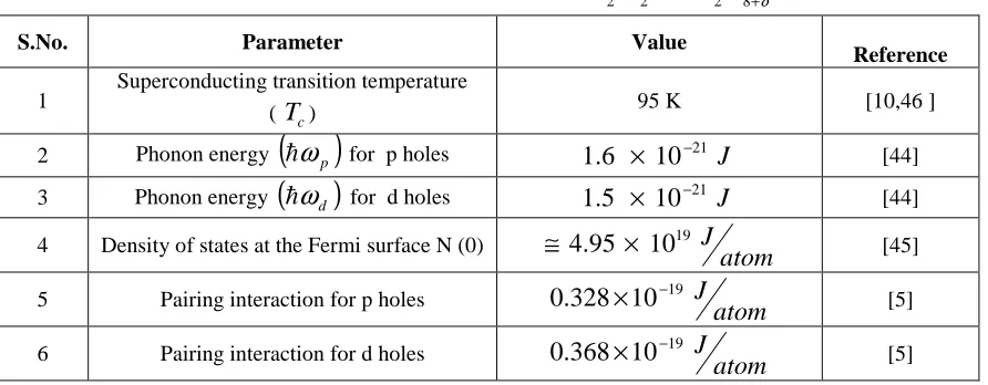
[image:10.595.87.533.582.756.2]

Values of various parameters appearing in equations obtained in the previous section are given in Table 1. Using these values, we have made study of various parameters for the system Bi₂Sr₂CaCu₂O_8+δ .

TABLE 1: VALUES OF VARIOUS PARAMETERS FOR Bi₂Sr₂CaCu₂O_8+δ SYSTEM

S.No. Parameter Value

Reference

1

Superconducting transition temperature

( T_c) 95 K [10,46 ]

2 Phonon energy

( )

hω_p for p holes _1.6 × ₁₀−21 _J [44]

3 Phonon energy

(

h

ω

_d

)

for d holes 21 J

10 5 .

1 × − [44]

4 Density of states at the Fermi surface N (0) ≅ 4.95 × 1019

atom

J _[45]

5 Pairing interaction for p holes

atom J 19 10 328 .

0 × − [5]

6 Pairing interaction for d holes

atom J 19 10 368 .

3.1 SUPERCONDUCTING ORDER PARAMETER

( )

∆

For the study of superconducting order parameter for Bi2Sr2CaCu2O8_+δ system with two

band model one finds three different situations: (i) The superconducting order parameter in the presence of p-holes only , (ii) The superconducting order parameter in the presence of d-holes only and (iii) The superconducting order parameter for both the d-holes.

(a) The SC order parameter for p-holes (BCS Type, in the absence of doping )

One obtains the expression for ∆p as

(

)

k

T

E

d

N

V

B

p p

pp

p

2

tanh

)

0

(

1

0 1 2

∫

₋

∈

=

ω

α

α

h

( 56 )

One can rewrite equation ( 56 ) as ,

T

k

d

N

V

B

p

pp

p p

p

p

p

2

tanh

2

1

)

0

(

1

2 2

0 2 2

∆

+

∈

∆

+

∈

∈

=

_∫

ω

h

( 57 )

Using the following changes in variables, and taking µ =0 in the absence of doping

J x

p

21

10−

× =

∆ ,∈_p=hω_py, d∈_p=hω_pdy ( 58 )

Equation ( 57 ) reduced to ,

∫





























































_×

+

















_×

+

=

− −

1

0 21 2

2

2 21 2

10

10

2

tanh

)

0

(

1

p p

B p

pp

_x

y

T

x

y

k

dy

N

V

ω

ω

ω

h

h

h

( 59 )

and taking the respective values from Table 1, one obtains 58

97 . 57

2kB = K ≅ p

ω

h

( 60 )

Using the above values and simplifying equation ( 60 ) , one obtains

7 Number of atoms per unit volume _~ 22

10

5× [45]

8 Boltzmann constant

( )

k_B 1.38 × 10−23 J K

9 Electron Mass

( )

m_e 9.1 10 31 .

Kg

−

∫

_















₊

+

=

1 0 2 2 2 2

3906

.

0

58

tanh

3906

.

0

)

0

(

1

T

x

y

x

y

dy

N

V

pp

( 61 )

Or

∫

_















+

−

+

+

=

+ + − 1

0 0.3906

116 3906 . 0 116 2 2

1

1

1

1

3906

.

0

6173

.

0

2 2 2

2 _{y x}

T x y T

_e

e

x

y

dy

( 62 )

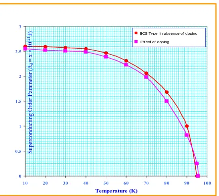
Solving equations ( 62 ) numerically, one can study the variation of SC order parameter with temperature in the absence of d-holes. The values obtained from equations ( 62 ) are depicted in Table 2 and the behavior is shown in Figure 1 for p holes .

(b) The SC order parameter for p-holes (Effect of doping )

Using equation ( 57 ) ,

T

k

d

N

V

B p pp p p p p p

2

tanh

2

1

)

0

(

1

2 2

0 2 2

∆

+

∈

∆

+

∈

∈

=

_∫

ω h

( 63 )

Using the following changes in variables

J x p 21 10− × =

∆ , ∈p=∈p0 −

µ

,

0

p p d

d∈ = ∈ ( 64 )

Equation ( 63 ) becomes ,

(

)

(

)

(

)

k

T

(

)

x

x

d

N

V

B p p p pp p

2

10

tanh

10

2

1

)

0

(

1

2 21 2 0 2 21 2 0 0 − + −

×

+

−

∈

×

+

−

∈

∈

=

_∫

µ

µ

ω µ

µ

h

( 65 )

Further changes in variables as

y p p =h

ω

∈ 0

, d∈p =h

ω

pdy

0

( 66 )

Equation ( 65 ) takes the following form

(

)

(

)

(

)

k

T

(

)

x

y

x

y

dy

N

V

B p p p pp p p

2

10

tanh

10

2

1

)

0

(

1

2 21 2 1 2 21 2 − + −

×

+

−

×

+

−

=

_∫

ω

µ

µ

ω

ω

ω µ ω µ

h

h

h

h h

( 67 )

Taking the following values,

J p 21 10 6 .

1 × −

≅

ω

h

[image:13.595.63.513.185.763.2]

Solving equations ( 62 ) and ( 67 ) numerically one can study the variation of superconductivity order parameter

( )

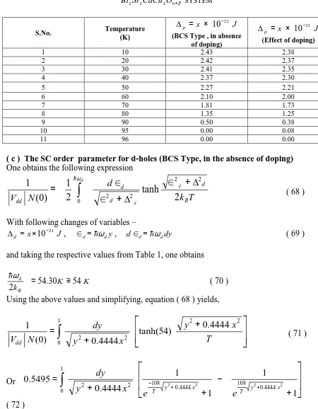
∆ with temperature in the absence of d-holes. The values obtained from equations ( 62 ) and ( 67 ) are depicted in Table 2 and the comparison of superconductivity order parameter for BCS type , in the absence of doping and effect of doping is shown in Fig. 1 for p holes.

TABLE 2: SUPERCONDUCTING ORDER PARAMETER

( )

∆_p ( p-HOLES) FOR

δ

+ 8 2 2

2Sr CaCu O

i

B SYSTEM

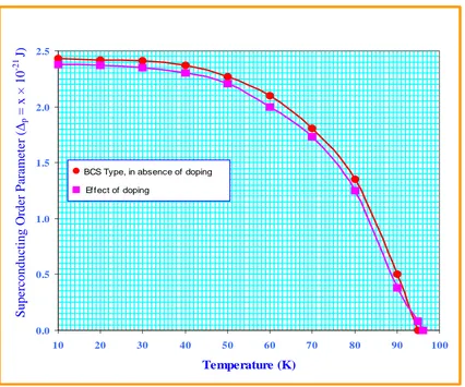
( c ) The SC order parameter for d-holes (BCS Type, in the absence of doping)

One obtains the following expression

T

k

d

N

V

B

d

d d

dd

d d

d

2

tanh

2

1

)

0

(

1

2 2

0 2 2

∆

+

∈

∆

+

∈

∈

=

ω

_∫

h

( 68 )

With following changes of variables –

J x

d

21

10−

× =

∆ , ∈d=h

ω

dy, d∈d=h

ω

ddy ( 69 )

and taking the respective values from Table 1, one obtains

K K

kB d

54 30

. 54

2 = ≅

ω

h

( 70 ) Using the above values and simplifying, equation ( 68 ) yields,

∫

_















₊

+

=

1

0

2 2

2 2

4444

.

0

)

54

tanh(

4444

.

0

)

0

(

1

T

x

y

x

y

dy

N

V

_dd ( 71 )

Or

∫

_















+

−

+

+

=

+ +

−

1

0 0.4444

108 4444

. 0 108 2

2

1

1

1

1

4444

.

0

5495

.

0

2 2

2

2 _{y x}

T x

y

T

_e

e

x

y

dy

( 72 )

S.No. Temperature (K)

J x

p

21

10−

× = ∆

(BCS Type , in absence of doping)

J x

p

21

10−

× = ∆

(Effect of doping)

1 10 2.43 2.38

2 20 2.42 2.37

3 30 2.41 2.35

4 40 2.37 2.30

5 50 2.27 2.21

6 60 2.10 2.00

7 70 1.81 1.73

8 80 1.35 1.25

9 90 0.50 0.38

10 95 0.00 0.08

[image:14.595.104.530.74.429.2]

Fig :1 Behavior of superconducting order parameter (∆_p) with temperature for p-holes.

(d) The SC order parameter for d-holes (Effect of doping )

Using equation ( 68 ) ,

T

k

d

N

V

B

d

dd

d d d

d

d

2

tanh

2

1

)

0

(

1

2 2

0 2 2

∆

+

∈

∆

+

∈

∈

=

_∫

ω

h

( 73 )

Using the following changes in variables

J x

d

21

10−

× =

∆ , ∈_d=∈_d0 −

µ

, d∈_d=d∈_d0 ( 74 )

Equation ( 73 ) becomes ,

(

)

(

)

(

)

k

T

(

)

x

x

d

N

V

B

d

d

d

dd

d

2

10

tanh

10

2

1

)

0

(

1

0 2 21 2

2 21 2

0

0 −

+

−

×

+

−

∈

×

+

−

∈

∈

=

_∫

µ

µ

ω µ

µ

h

( 75 ) 0.0 0.5 1.0 1.5 2.0 2.5

10 20 30 40 50 60 70 80 90 100

Temperature (K)

●

BCS Type, in absence of doping

■

Ef fect of doping

S

u

p

er

co

n

d

u

ct

in

g

O

rd

er

P

ar

am

et

er

(

∆p

=

x

×

1

0

-2

Further changes in variables as

y

d d =h

ω

∈ 0

, d∈_d0=h

ω

_ddy ( 76 )

Equation ( 75 ) takes the following form

(

)

(

)

(

)

(

)

T

k

x

y

x

y

dy

N

V

B

d

d

d dd

d

d

2

10

tanh

10

2

1

)

0

(

1

2 21 2

1

2 21 2

− +

−

×

+

−

×

+

−

=

_∫

ω

µ

µ

ω

ω

ω µ

ω µ

h

h

h

h

h

( 77 ) Taking the following values,

J d

21

10 5 .

1 × −

≅

ω

h

K J kB

23

10 38 .

1 × −

=

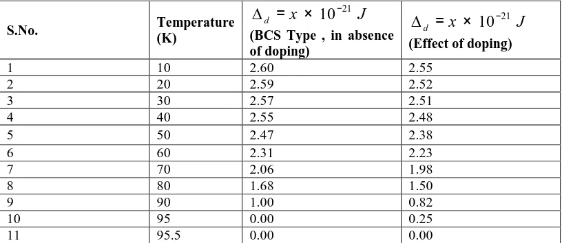
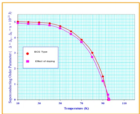
[image:15.595.122.530.433.610.2]

Solving equations ( 72 ) and ( 77 ) numerically one can study the variation of superconducting order parameter with temperature in the absence of p-holes. The values obtained from equations ( 72 ) and ( 77 ) are depicted in Table 3 and the comparison of superconductivity order parameter for BCS type, in the absence of doping and effect of doping for d holes is shown in Fig. 2.

TABLE 3: SUPERCONDUCTING ORDER PARAMETER

( )

∆_d ( d-HOLES) FOR Bi₂Sr₂CaCu₂O_8+δ SYSTEM

S.No. Temperature (K)

J x

d

21

10−

× = ∆

(BCS Type , in absence of doping)

J x

d

21

10−

× = ∆

(Effect of doping)

1 10 2.60 2.55

2 20 2.59 2.52

3 30 2.57 2.51

4 40 2.55 2.48

5 50 2.47 2.38

6 60 2.31 2.23

7 70 2.06 1.98

8 80 1.68 1.50

9 90 1.00 0.82

10 95 0.00 0.25

[image:16.595.79.522.72.467.2]

Fig :2 Behavior of superconducting order parameter (∆_d) with temperature for d-holes. TABLE 4: SUPERCONDUCTING ORDER PARAMETER

(

∆=∆_p +∆_d

)

( p & d HOLES)

FOR Bi₂Sr₂CaCu₂O_8+δ SYSTEM

S.No. Temperature

(K)

) (∆ =∆_p +∆_d

Joule

x 21

10−

× =

(BCS Type , in absence of doping)

) (∆=∆_p +∆_d

Joule x × 10−21

=

(Effect of doping)

1 10 5.03 4.93

2 20 5.01 4.89

3 30 4.98 4.86

4 40 4.92 4.78

5 50 4.74 4.59

6 60 4.41 4.23

7 70 3.87 3.71

8 80 3.03 2.75

9 90 1.50 1.20

10 95 0.00 0.33

11 95.5 0.00 0.07

12 96 0.00 0.00

0 0.5 1 1.5 2 2.5 3

10 20 30 40 50 60 70 80 90 100

Temperature (K)

●

BCS Type, in absence of doping

■

Effect of doping

S

u

p

er

co

n

d

u

ct

in

g

O

rd

er

P

ar

am

et

er

(

∆d

=

x

×

1

0

-2

[image:17.595.96.555.67.440.2]

Fig :3 Behavior of superconducting order parameter (∆=∆_p +∆_d) with temperature For p and d-holes.

( e ) SC order parameter in the presence of both p and d holes

The superconducting order parameter in the presence of both holes can be studied by taking a simple sum of both the parameters. Taking the sum of order parameter as

(

∆=∆p +∆d

)

one can obtain the values by solving numerically as depicted in Table 4 and the comparison of superconductivity order parameter for BCS type, in the absence of doping and effect of doping for both p and d holes is shown in Fig. 3.

3.2 DEPENDENCE OF CHEMICAL POTENTIAL

( )

µ

ON CRITICAL TEMPERATURE

( )

T c

For Bi₂Sr₂CaCu₂O_8+δ superconductors, we used the best fitting parameters values for numerical estimation as follows :

1

210 . 0 )

0

( =densityof states for pholes= eV−

N_p ,

1

045 . 0 )

0

( =densityof states for d holes= eV−

Nd ,

eV bands

two between erchange

pair The

V_pd = int =1.65 ,

eV band

lower of energy off

Cut

c= − = 2.33

∈ ,

eV width

the of band higher of

energy

top 2.5

1= =

∈ ,

0 1 2 3 4 5

10 30 50 70 90 110

Temperature (K)

BCS Type

Effect of doping

S

u

p

er

co

n

d

u

ct

in

g

O

rd

er

P

ar

am

et

er

(

∆

=

∆p

+

∆d

=

x

×

1

0

-2

eV band

lower of energy

top 2.18

0= =

∈ ,

eV Joule

p 1.6 10 0.010

21 = × = −

ω

h _, eV Joule

d 1.5 10 0.009375

21 =

×

= −

ω

h .

The small difference between ∈_c and ∈₀ is taken keeping in mind the uncertainty in defining the effective bottom of the band∈_c.

The parameters are model dependent for the calculation of Tc

( )

n . These quantitative h characteristic seem to be reasonable at least they are of the order proposed by Konsin and coworkers [10,26] for high T cuprates. _c

Applying the limits of integration on equation ( 53 ), for dependence of transition temperature

( )

T on chemical potential c

( )

µ

dependence, one obtains

1

2

tanh

2

tanh

)

0

(

)

0

(

2

∈

=

∈

∈

×

∈

∈

∈

∫

∫

c B p p p c B d d d d p pd

T

k

d

T

k

d

N

N

V

Or,

1

2

tanh

2

tanh

02572

.

0

33 . 2 18 . 2 33 . 2

=

∈

∈

∈

×

∈

∈

∈

∫

∫

− − −

− B c

p p p c B d d d

T

k

d

T

k

d

µ µ µ

µ ( 78 )

Solving numerically equation ( 78 ) , we obtain values given in Table 5 for T with respect _c

to different doping parameters

( )

µ

.

3.3 DEPENDENCE OF CRITICAL TEMPERATURE (T ) ON HOLE _c

CONCENTRATION

( )

n _h

By substituting numerical values of chemical potential µ and Critical temperature T _c

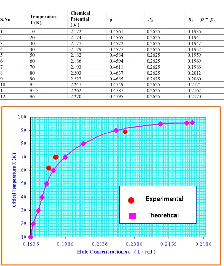
obtained from equation ( 78 ) in equation ( 55 ) with relevant parameters , we obtain dependence of critical temperature T , on hole concentration _c n . _h

Using equation ( 55 ), we obtain dependence of Critical temperature T on hole concentration c

( )

n for system h Bi2Sr2CaCu2O8+δ as shown in Table 5 and depicted in Fig. 4.

p B c B B c N B B B N

T

k

T

k

T

k

T

k

T

k

T

k

d

p + =

[image:19.595.71.528.105.647.2]

TABLE 5: DEPENDENCE OF CRITICAL TEMPERATURE

( )

T_c ON HOLE CONCENTRATION

( )

n_h

Fig : 4 Variation of Critical Temperature

( )

T_c with Hole Concentration

( )

n_h [10].

DISCUSSION AND CONCLUSION

In the foregoing sections, we have presented the study of photo-induced high T cuprate c superconductivity by canonical two-band BCS Hamiltonian containing Fermi surfaces of p and d holes.

S.No. Temperature T (K)

Chemical Potential (µ)

p po nh = p− p0

1 10 2.172 0.4561 0.2625 0.1936

2 20 2.174 0.4565 0.2625 0.194

3 30 2.177 0.4572 0.2625 0.1947

4 40 2.179 0.4577 0.2625 0.1952

5 50 2.182 0.4584 0.2625 0.1959

6 60 2.186 0.4594 0.2625 0.1969

7 70 2.193 0.4611 0.2625 0.1986

8 80 2.203 0.4637 0.2625 0.2012

9 90 2.222 0.4685 0.2625 0.2060

10 95 2.247 0.4749 0.2625 0.2124

11 95.5 2.262 0.4787 0.2625 0.2162