Detection of Structural Changes in Correctly Specified and Misspecified Conditional Quantile Polynomial Distributed Lag (QPDL) Model Using Change point Analysis

Detection of Structural Changes in Correctly Specified

and Misspecified Conditional Quantile Polynomial

Distributed Lag (QPDL) Model Using

Change-point Analysis

Kwadwo Agyei Nyantakyi

_{, B. L. Peiris, L. H. P. Gunaratne}

Postgraduate Institute of Agriculture, University of Peradeniya, Sri Lanka

Copyright © 2015 Horizon Research Publishing All rights reserved.

Abstract

determining whether a change has taken place or not. In this paper we study the structural changes in the Conditional Quantile Polynomial Distributed Lag (QPDL) model using change-point analysis. We employ both the Binary Segmentation (BinSeg) and Cumulative Sum (Cusum) methods for this analysis. We studied the structural changes in both correctly specified and misspecified QPDL models. As an economic application we considered the production of rubber and its price returns. We observe that both Cusum and BinSeg methods correctly detected the structural changes for both the correctly specified and the misspecified QPDL model. The Cusum method gave the exact positions where the structural changes occurred and the BinSeg gave the approximated positions where the changes occurred. Both methods were able to detect the shift in time for both the mean and variance for the missspecified QPDL model, hence both methods were better for predicting structural stability in a QPDL models. The impact of this is that, when there are changes made to a data knowingly or unknowingly, they can be detected, as well as when these changes were effected. We further observed that both methods were powerful tools that better characterizes the changes, controls the overall error rate, robust to outliers, more flexible and simple to use.

Keywords

Misspecification, Mean-shift

1. Introduction

The question of structural stability of models is very important in predicting the future in various diverse areas of science such as economics, finance, physics, geology, medicine as well as in quality control and agriculture. Questions like did a change occur? Did more than one

change occur? When did these changes occur? Can be answered by performing a change-point analysis, (Taylor, Wayne 2000a, 2000b)[13, 14].

In order to study the structural changes in models came the evolution of change-points which was introduced by the context of quality control by Csorgo and Horvath, (1997)[3]. Change–points has been employed in finding the possible changes in otherwise independent identically distributed random variables and has been extended to the stability tests of parameters of the regression functions, (Andrews, D. W. K. 1993)[1].

Killick, et al, (2012)[9], considered the common approach of detecting change-points through minimising a cost function over possible numbers and locations of change-points. They applied several established procedures for detecting changing points, such as penalised likelihood and minimum description length. In their study, they observed that Binary Segmentation is quicker as a search method, and believed this would be the case in almost all applications.

Auger and Lawrence (1989)[2] propose an alternative, exact search method for changepoint detection, namely the Segment Neighbourhood (SegNeigh) method which searches the entire segmentation space using dynamic programming. The problem with this exhaustive search method is that it has significant computational cost of

Ο(𝑄𝑄𝑛𝑛2).

The objectives of this study are, to detect the structural changes in correctly specified QPDL model, to detect the structural changes in misspecified QPDL model, and to study the mean-shift in time of the misspecified QPDL model. This study is important because as the part of our world moves into more sophisticated time periods, the accuracy of predicting the exact occurrences of future events as much as possible to reduce severe loses or impact is very important rather than using approximate estimates. It is also important in modeling to know when the exact change occurred and its impact.

2. Materials and Methods

2.1. Data Source

In order to answer the issues raised above, secondary annual data was collected from FAOSTAT, food balance sheet, price statistics, available with the Department of Census and Statistics Sri Lanka[6], and the World Bank (pink sheet)[15]. These data comprises of the production, imports, exports and prices of rubber. The rubber data ranges from 1961-2011.

2.2. Statistical Software

The R software, with the package ‘Change-point’ was used in analysing the structural changes in the conditional quantile polynomial distributed lag models.

2.3. Methodology

Testing for structural changes

We assume two (2) conditional 2nd _{degree polynomial}

𝛼𝛼 − 𝑞𝑞𝑞𝑞𝑞𝑞𝑞𝑞𝑞𝑞𝑞𝑞𝑞𝑞𝑞𝑞 regimes

𝑌𝑌1𝑡𝑡= 𝜑𝜑(𝛼𝛼) + 𝑞𝑞1,0(𝛼𝛼)𝑍𝑍1,0𝑡𝑡+ 𝑞𝑞1,1(𝛼𝛼)𝑍𝑍1,1𝑡𝑡+ 𝑞𝑞1,2(𝛼𝛼)𝑍𝑍1,2𝑡𝑡

+𝜀𝜀1𝑡𝑡, 𝑞𝑞 = 1,2, … , 𝑇𝑇1 (1) 𝑌𝑌2𝑡𝑡= 𝜑𝜑(𝛼𝛼) + 𝑞𝑞2,0(𝛼𝛼)𝑍𝑍2,0𝑡𝑡+ 𝑞𝑞2,1(𝛼𝛼)𝑍𝑍2,1𝑡𝑡

+𝑞𝑞2,2(𝛼𝛼)𝑍𝑍2,2𝑡𝑡, +𝜀𝜀2𝑡𝑡, 𝑞𝑞 = 1,2, … , 𝑇𝑇2 (2)

With {𝜀𝜀1𝑡𝑡} and {𝜀𝜀1𝑡𝑡} i.i.d unobservable innovations with 𝐸𝐸(𝜀𝜀1𝑡𝑡) = 0 𝑞𝑞𝑞𝑞𝑎𝑎 𝐸𝐸(𝜀𝜀2𝑡𝑡) = 0 , 𝑉𝑉(𝜀𝜀1𝑡𝑡)

= 𝜎𝜎12 𝑞𝑞𝑞𝑞𝑎𝑎 𝑉𝑉(𝜀𝜀2𝑡𝑡) = 𝜎𝜎22

We further assume that 𝐸𝐸(𝜀𝜀1𝑡𝑡) 𝑞𝑞𝑞𝑞𝑎𝑎 𝐸𝐸(𝜀𝜀2𝑡𝑡) are i.i.d

innovations which are independent of each other.

Let 𝑞𝑞�1,0(𝛼𝛼) and 𝑞𝑞�2,0(𝛼𝛼) be the estimates of

𝑞𝑞1,0(𝛼𝛼) 𝑞𝑞𝑞𝑞𝑎𝑎 𝑞𝑞2,0(𝛼𝛼) respectively. Then we also define

𝑌𝑌1𝑡𝑡∗ = 𝑌𝑌1𝑡𝑡− 𝑌𝑌�1 𝑞𝑞𝑞𝑞𝑎𝑎 𝑌𝑌2𝑡𝑡∗ = 𝑌𝑌2𝑡𝑡− 𝑌𝑌�1

Then the hypothesis can be tested as follows: Hypothesis:

𝐻𝐻0: 𝑞𝑞1,0(𝛼𝛼) = 𝑞𝑞2,0(𝛼𝛼)𝑞𝑞𝑞𝑞𝑎𝑎 𝐻𝐻1: 𝑞𝑞1,0(𝛼𝛼) ≠ 𝑞𝑞2,0(𝛼𝛼)

(Assuming 𝜎𝜎12= 𝜎𝜎22)

Then under 𝐻𝐻0 we have,

� 𝜎𝜎12

∑𝑻𝑻𝟏𝟏_{𝒕𝒕=𝟏𝟏}�𝑌𝑌_1𝑡𝑡∗�𝟐𝟐+ 𝜎𝜎12

∑𝑻𝑻𝟐𝟐_{𝒕𝒕=𝟏𝟏}�𝑌𝑌_2𝑡𝑡∗�𝟐𝟐� −𝟏𝟏 𝟐𝟐⁄

�𝑞𝑞�1,0(𝛼𝛼) − 𝑞𝑞�2,0(𝛼𝛼)� ~𝑵𝑵(𝟎𝟎, 𝟏𝟏)

(3) Let (𝜀𝜀̂1𝑡𝑡) 𝑞𝑞𝑞𝑞𝑎𝑎 (𝜀𝜀̂2𝑡𝑡) be the residuals estimated

respectively, then ∑𝑻𝑻𝟏𝟏𝒕𝒕=𝟏𝟏𝜺𝜺�𝟏𝟏𝒕𝒕𝟐𝟐

𝜎𝜎12 ~𝝌𝝌𝒕𝒕−𝟐𝟐

𝟐𝟐 _{𝒂𝒂𝒂𝒂𝒂𝒂} ∑𝑻𝑻𝟐𝟐𝒕𝒕=𝟏𝟏𝜺𝜺�𝟐𝟐𝒕𝒕𝟐𝟐

𝜎𝜎22 ~𝝌𝝌𝒕𝒕−𝟐𝟐

𝟐𝟐

and therefore we have

∑𝑻𝑻𝟏𝟏𝒕𝒕=𝟏𝟏𝜺𝜺�𝟏𝟏𝒕𝒕𝟐𝟐

𝜎𝜎₁2 +

∑𝑻𝑻𝟐𝟐𝒕𝒕=𝟏𝟏𝜺𝜺�𝟐𝟐𝒕𝒕𝟐𝟐

𝜎𝜎₂2 ~𝝌𝝌𝒕𝒕−𝟒𝟒𝟐𝟐 (4)

Where we have 𝑻𝑻𝟏𝟏+ 𝑻𝑻𝟐𝟐= 𝑻𝑻 and since (3) and (4) are

independent we have

√𝑇𝑇−4�𝑎𝑎�1,0(𝛼𝛼)− 𝑎𝑎�2,0(𝛼𝛼) �

� 𝜎𝜎12

∑𝑻𝑻𝟏𝟏_{𝒕𝒕=𝟏𝟏�𝑌𝑌1𝑡𝑡}∗ �𝟐𝟐+ 𝜎𝜎12 ∑𝑻𝑻𝟐𝟐_{𝒕𝒕=𝟏𝟏�𝑌𝑌2𝑡𝑡}∗ �𝟐𝟐�

𝟏𝟏 𝟐𝟐⁄

�∑𝑻𝑻𝟏𝟏𝒕𝒕=𝟏𝟏𝜺𝜺�𝟏𝟏𝒕𝒕𝟐𝟐

𝜎𝜎12 + ∑𝑻𝑻𝟐𝟐_{𝒕𝒕=𝟏𝟏𝜺𝜺�𝟐𝟐𝒕𝒕}𝟐𝟐

𝜎𝜎22 �

𝟏𝟏 𝟐𝟐⁄ ~𝑞𝑞𝑇𝑇−4 and

since 𝜎𝜎12= 𝜎𝜎22 we have �𝑎𝑎�1,0(𝛼𝛼)− 𝑎𝑎�2,0(𝛼𝛼) �

� 𝜎𝜎12

∑𝑻𝑻𝟏𝟏_{𝒕𝒕=𝟏𝟏�𝑌𝑌1𝑡𝑡}∗ �𝟐𝟐+ 𝜎𝜎12 ∑𝑻𝑻𝟐𝟐_{𝒕𝒕=𝟏𝟏�𝑌𝑌2𝑡𝑡}∗ �𝟐𝟐�

1 2⁄ ~𝑞𝑞𝑇𝑇−4 where

𝜎𝜎�2_{= (𝑇𝑇 − 4)}2_{�∑ 𝜺𝜺�} 𝟏𝟏𝒕𝒕 𝟐𝟐 𝑻𝑻𝟏𝟏

𝒕𝒕=𝟏𝟏 + ∑𝑻𝑻𝒕𝒕=𝟏𝟏𝟐𝟐 𝜺𝜺�𝟐𝟐𝒕𝒕𝟐𝟐� (5)

Hence 𝐻𝐻0 can be tested using either one tail or two tail

depending on the 𝐻𝐻1.

Now we apply the change point algorithm to see when and where the changes in the QPDL model occurred, using cumulative sum (cusum) and Binary Segmentation (BinSeg) methods.

Description of the test procedure for the detection of the change-point

Let us now consider a conditional 2nd _{degree polynomial}

𝛼𝛼 − 𝑞𝑞𝑞𝑞𝑞𝑞𝑞𝑞𝑞𝑞𝑞𝑞𝑞𝑞𝑞𝑞 model with a change after an unknown time point

1 ≤ 𝑘𝑘∗_{= 𝑘𝑘}∗_{(𝑞𝑞) ≤ 𝑞𝑞}

𝑋𝑋𝑖𝑖𝑡𝑡= �𝑍𝑍𝑖𝑖𝑡𝑡 𝑞𝑞 ≤ 𝑘𝑘 ∗

𝑌𝑌𝑖𝑖𝑡𝑡−𝑘𝑘∗ 𝑞𝑞 > 𝑘𝑘∗ (6) Where {𝑌𝑌𝑖𝑖𝑡𝑡} is some QPDL which differs distributionally

from {𝑍𝑍𝑖𝑖𝑡𝑡}. The unknown parameter 𝑘𝑘∗ is called the

change-point.

We are now interested in the testing problem

𝐻𝐻 0: 𝑘𝑘∗= 𝑞𝑞 vs. 𝐻𝐻 1: 𝑘𝑘∗< 𝑞𝑞

Our testing procedures are based on various functionals of the partial sums of estimated

residuals with respect to the model (1)

𝑆𝑆̂𝑞𝑞(𝑘𝑘) = � 𝜀𝜀̂𝑡𝑡 𝑘𝑘

𝑡𝑡=𝑝𝑝+1

=∑𝑘𝑘𝑡𝑡=𝑝𝑝+1�𝑋𝑋𝑖𝑖𝑡𝑡− 𝑓𝑓�𝑍𝑍𝑖𝑖𝑡𝑡, 𝛽𝛽̂𝑛𝑛��. (7)

where 𝛽𝛽̂𝑛𝑛 is the least-squares estimator of 𝛽𝛽0 (assuming the

null hypothesis holds true).

𝑄𝑄𝑛𝑛(𝛽𝛽) = � �𝑋𝑋𝑡𝑡− 𝑓𝑓�𝑍𝑍𝑖𝑖𝑡𝑡, 𝛽𝛽̂𝑛𝑛�� 2 𝑘𝑘

𝑡𝑡=𝑝𝑝+1

=∑𝑘𝑘𝑡𝑡=𝑝𝑝+1𝑞𝑞𝑛𝑛(𝛽𝛽) (8)

Thus we consider the nonlinear least squares estimator

𝛽𝛽̂𝑛𝑛= 𝑞𝑞𝑎𝑎𝑎𝑎 min𝛽𝛽𝛽𝛽𝑘𝑘𝑄𝑄𝑛𝑛(𝛽𝛽) (9)

for a suitable compact set K. The minimization is usually obtained by solving the nonlinear score function

𝜕𝜕𝑄𝑄𝑛𝑛(𝛽𝛽�𝑛𝑛)

𝜕𝜕𝛽𝛽 = 0. (10)

Which yields

∑𝑘𝑘𝑡𝑡=𝑝𝑝+1𝜀𝜀̂𝑡𝑡= 0. (11)

The behaviour of the estimator 𝛽𝛽𝑛𝑛 is investigated in a

variety of situations including the correctly specified case without change as well as possibly misspecified cases with and without change. According to Horvath et al (2004)[8] and Wu, (2004)[16], under appropriate assumptions 𝛽𝛽̂𝑛𝑛 is

eventually in the interior of the compact set K, so that we can assume for limit considerations.

In fact, if 𝛽𝛽̂𝑛𝑛 is not in the interior of K, (Hinkley, D. V.

1971)[7], we will reject the null hypothesis immediately since either a change occurred or the model is not capable of modeling the observed time series sufficiently well.

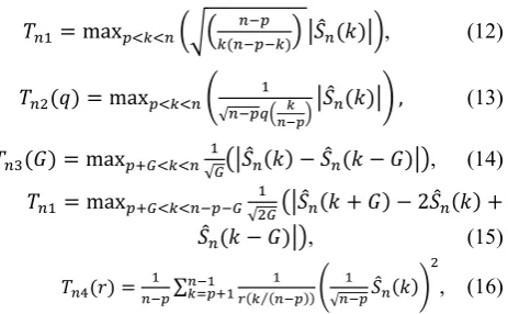
Test statistics are of the form

𝑇𝑇𝑛𝑛1= max𝑝𝑝<𝑘𝑘<𝑛𝑛���_{𝑘𝑘(𝑛𝑛−𝑝𝑝−𝑘𝑘)}𝑛𝑛−𝑝𝑝 � �𝑆𝑆̂𝑛𝑛(𝑘𝑘)��, (12)

𝑇𝑇𝑛𝑛2(𝑞𝑞) = max𝑝𝑝<𝑘𝑘<𝑛𝑛� 1

√𝑛𝑛−𝑝𝑝𝑞𝑞�_{𝑛𝑛−𝑝𝑝}𝑘𝑘 ��𝑆𝑆̂𝑛𝑛(𝑘𝑘)�� , (13)

𝑇𝑇𝑛𝑛3(𝐺𝐺) = max𝑝𝑝+𝐺𝐺<𝑘𝑘<𝑛𝑛_√𝐺𝐺1��𝑆𝑆̂𝑛𝑛(𝑘𝑘) − 𝑆𝑆̂𝑛𝑛(𝑘𝑘 − 𝐺𝐺)��, (14)

𝑇𝑇𝑛𝑛1= max𝑝𝑝+𝐺𝐺<𝑘𝑘<𝑛𝑛−𝑝𝑝−𝐺𝐺_√2𝐺𝐺1 ��𝑆𝑆̂𝑛𝑛(𝑘𝑘 + 𝐺𝐺) − 2𝑆𝑆̂𝑛𝑛(𝑘𝑘) +

𝑆𝑆̂𝑛𝑛(𝑘𝑘 − 𝐺𝐺)��, (15)

𝑇𝑇𝑛𝑛4(𝑎𝑎) =_{𝑛𝑛−𝑝𝑝}1 ∑ _{𝑟𝑟(𝑘𝑘 (𝑛𝑛−𝑝𝑝)⁄}1 ₎�_{√𝑛𝑛−𝑝𝑝}1 𝑆𝑆̂𝑛𝑛(𝑘𝑘)� 2 𝑛𝑛−1

𝑘𝑘=𝑝𝑝+1 , (16)

where q(·) and r(·) are weight functions defined on (0,1) specified below and G < n. In this case, we obtain a consistent change-point estimator which is related to the test statistics. (Stockis, J.-P et al, 2010, Tadjuidje K., J. et al, 2011)[11, 12]

3. Results and Discussions

Detection of structural Changes for the correctly specified QPDL model

Detection of structural changes in the QPDL model before misspecification are shown on tables 1 - 4, using the methods Cumulative Sum (cusum) and Binary Segmentation (BinSeg) with Schwarz Information Criterion (SIC) penalty.

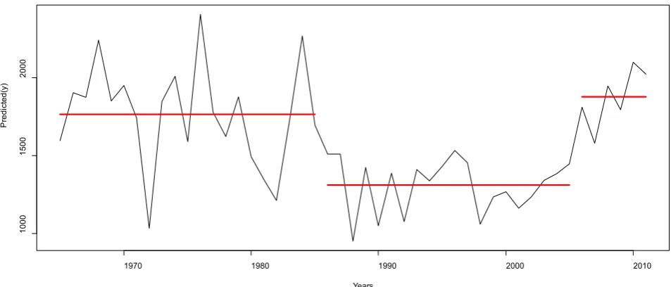
Figure 1. a plot showing the changes in production of Predicted 𝑦𝑦� against Years of tau=0.25

Table 1. Conditional quantile polynomial distributed lag (QPDL), tau=0.25 showing the maximum number of changes, position of the change in both the mean and variance for cusum and BinSeg methods. (SIC (Penalty) = 7.742402)

tau Change type Positions of the change Max no. of change

0.25 Cusum 16.00 41.00 44.00 46.00 24.00 5

BinSeg 16 19 23 42 44 48 5

Mean 1572.5 1000.9 1539.4 1028.4 1432.9 1829.5

Variance 52268.88 42726.38 36481.89 22493.61 570.39 30727.15

Changepoint at tau(0.25)

Years

P

redi

ct

ed(

y)

1970 1980 1990 2000 2010

800

1000

1200

1400

1600

1800

From table 1, we observe that, both the cumulative sum (Cusum) and the Binary Segmentation (BinSeg) methods detected maximum of 5 structural changes. The Cusum gives the exact change at various positions whereas the BinSeg gives the approximated positions. The minimum change for both methods is at the 16th _{position and the highest maximum} for Cusum is 46th _{and that of BinSeg is 48}th _{position. There} changes in mean production with minimum of 1000.9, occurring at 19th _{position and the maximum mean of 1829.5} with a change at 48th _{position. The variance changes} associated with the changes are shown in the last row with minimum variance of 570.4 and for a mean of 1432.9 at the 44th _{position and a maximum variance of 52268.9 for a mean} of 1572.5 at the 16th _{position. figure 1 showing the various} positions and the time period for which each change occurred.

From figure 1, we observe the 1st _{change occurred in 1979,} showing a high drop in average production to a record low. The 2nd _{change in production occurred in 1982 with a high} increase in average production again. The 3rd _{change shows} another drop in average production which lasted from 1977

to 2005 and then the 4th _{change in average production} occurred. There was an increase in average production from 2005 to 2008 and then a change occurred, and then a subsequent increase till 2011.

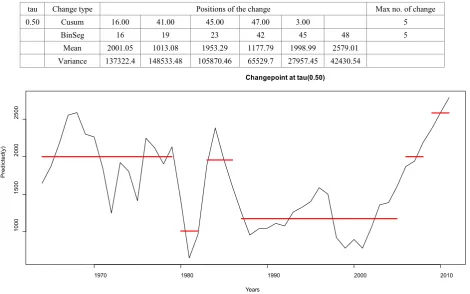
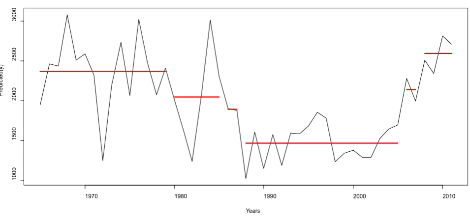
Table 2, we observed that, both methods detected 5 optimum changes, with the 1st _{change occurring at the 16}th position for both methods. The minimum average change in production 1013.1 occurred at 19th _{position with a variance} of 148533.5 and the highest average mean production 2579 occurred at 48th _{position with variance of 42430. The} graphical interpretation of the change is shown on figure 2.

Similarly, we observe from figure 2, the 1st _change occurred in 1979, showing a high drop in average production to a record low. The 2nd _{change in production occurred in} 1982 with a high increase in average production again. The 3rd _{change shows another drop in average production which} lasted from 1977 to 2005 and then the 4th _{change in average} production occurred. There was an increase in average production from 2005 to 2008 and then a change occurred, and then a subsequent increase till 2011.

Table 2. Conditional quantile polynomial distributed lag (QPDL) tau=0.50 showing the maximum number of changes, position of the change in both the mean and variance for cusum and BinSeg methods. (SIC (Penalty) = 7.742402)

tau Change type Positions of the change Max no. of change

0.50 Cusum 16.00 41.00 45.00 47.00 3.00 5

BinSeg 16 19 23 42 45 48 5

Mean 2001.05 1013.08 1953.29 1177.79 1998.99 2579.01

Variance 137322.4 148533.48 105870.46 65529.7 27957.45 42430.54

Figure 2 . a plot showing the changes in production of Predicted 𝑦𝑦� against Years of tau=0.50

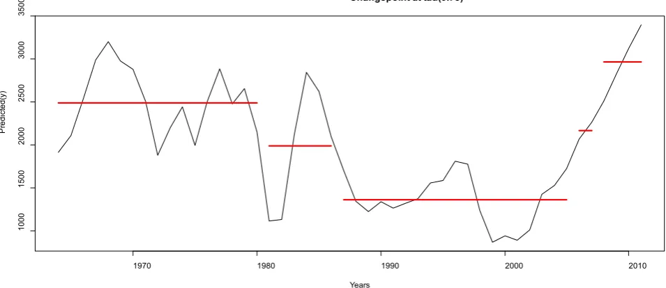
Table 3. Conditional quantile polynomial distributed lag (QPDL) tau=0.75 showing the maximum number of changes, position of the change in both the mean and variance for cusum and BinSeg methods. (SIC (Penalty) = 7.742402)

tau Change type Positions of the change Max no. of change

0.75 Cusum 17.00 42.00 45.00 24.00 19.00 5

BinSeg 17 23 42 44 48 4

Mean 2488.207 1987.198 1362.633 2166.128 2965.220

Variance 164495.50 533186.09 86739.77 18553.91 146672.70

Changepoint at tau(0.50)

Years

P

redi

ct

ed(

y)

1970 1980 1990 2000 2010

1000

1500

2000

Figure 3. a plot showing the changes in production of Predicted 𝑦𝑦� against Years of tau=0.75

Figure 4. a plot showing the changes in production of Predicted 𝑦𝑦� against Years of tau=0.95

Table 4 . Conditional quantile polynomial distributed lag (QPDL) tau=0.95 showing the maximum number of changes, position of the change in both the mean and variance for cusum and BinSeg methods. (SIC (Penalty) = 7.742402)

tau Change type Positions of the change Max no. of change

0.95 Cusum 23.000 42.000 45.000 46.000 17.000 5

BinSeg 17 24 32 43 45 48 5

Mean 3311.961 2586.547 1728.211 1654.949 2978.641 4032.445

Variance 313650.7 773252.0 33320.35 309450.68 33541.0 164135.34

Table 3 shows an optimum of 5 changes for Cusum and 4 for BinSeg. The minimum average production 1362.6 occurred at the 42nd _{position with a variance of 86739.8 and} the maximum average production 2965.2 occurring at the 48th _{position with variance of 146672.7. The graphical} interpretation is shown by figure 3.

We observe from figure 3, the 1st _{change occurred in 1981,} with a drop in average production between 1981 and 1986. The 2nd _{change in average production occurred in 1986 and} 2005 with a high decrease in average production again. The

3rd _{change shows another an average increase in production} which lasted from 2005 to 2007 and then the 4th _{change in} average production occurred. There was an increase in average production from 2005 till 2011.

Table 4, we observed that, both methods detected 5 optimum changes, with the 1st _{change occurring at the 23}rd position for Cusum and 17th _{position for BnSeg. The} minimum average change in production was 1655.1 and occurred at 43rd _{position with a variance of 309451 and the} highest average mean production was 4032.4 and occurred at

Changepoint at tau(0.75)

Years

P

redi

ct

ed(

y)

1970 1980 1990 2000 2010

1000

1500

2000

2500

3000

3500

Changepoint at tau(0.95)

Years

P

redi

ct

ed(

y)

1970 1980 1990 2000 2010

1000

1500

2000

2500

3000

3500

4000

48th _{position with variance of 164135. The graphical} interpretation of the change is shown on figure 4.

Similarly, we observe from figure 2, the 1st _change occurred in 1980, showing a drop in average production between 1980 and 1988. The 2nd _{change in production} occurred in 1988 with a further decrease in average production. The 3rd _{change shows another slight drop in} average production which lasted from 1997 to 2006 and then the 4th _{change in average production occurred. There was an} increase in average production from 2006 to 2008 and then a change occurred, and then a subsequent increase till 2011. Detection of structural Changes for the misspecified QPDL model

Detection of structural changes in the misspecified QPDL model are shown in tables 5 - 8, using the methods Cumulative Sum (cusum) and Binary Segmentation (BinSeg) with Schwarz Information Criterion (SIC) penalty.

From table 5, we observe that, both the cumulative sum

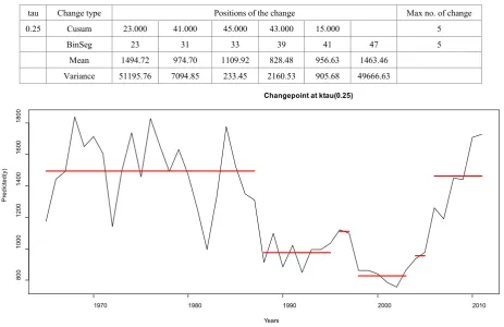
(Cusum) and the Binary Segmentation (BinSeg) methods detected maximum of 5 structural changes. Here there is a shift in position of the 1st _{change from the 16}th _{position from} the correctly specified model to 23rd _{position for the} misspecified model for both methods. The minimum change in mean production was 828.48, occurring at 39th _position with variance of 2161. The maximum average production of 1494.7 with a variance of 51195.8 occurred at 23rd _position. Below is figure 5 showing the various positions and the time period for which each change occurred.

Similarly, from figure 5, we observe a shift of the change in the average production which occurred in 1979 for the correctly specified QPDL model to 1988 in the misspecified QPDL model. There was high drop in the mean production between 1988 and 1996 and then an increase occurred for a short period in 1997. There was a drop again between 1998 and 2003. There was an increase in average production in 2004. There was a further high increase in production from 2005 till 2011.

Table 5. Misspecified Conditional quantile polynomial distributed lag (QPDL), tau=0.25 showing the maximum number of changes, position of the change in both the mean and variance for cusum and BinSeg methods. SIC (Penalty)= 7.700295

tau Change type Positions of the change Max no. of change

0.25 Cusum 23.000 41.000 45.000 43.000 15.000 5

BinSeg 23 31 33 39 41 47 5

Mean 1494.72 974.70 1109.92 828.48 956.63 1463.46

Variance 51195.76 7094.85 233.45 2160.53 905.68 49666.63

Figure 5. a plot showing the changes in production of Predicted 𝑦𝑦� against Years of tau=0.25

Table 6. Conditional quantile polynomial distributed lag (QPDL) misspecified tau=0.50 showing the maximum number of changes, position of the change in both the mean and variance for cusum and BinSeg methods. SIC (Penalty)= 7.700295

tau Change type Positions of the change Max no. of change

0.50 Cusum 21.000 40.000 43.000 41.000 42.000 5

BinSeg 21 41 47 3

Mean 1766.641 1311.461 1877.811

Variance 111066.87 30018.25 34896.11

Changepoint at ktau(0.25)

Years

P

redi

ct

ed(

y)

1970 1980 1990 2000 2010

800

1000

1200

1400

1600

Similarly, from table 6, we observe that, for the misspecified QPDL model, the cumulative sum (Cusum) detected a maximum of 5 structural changes and the Binary Segmentation (BinSeg) methods detected only 3 structural changes at the 50th _{percentile. Whereas in the correctly} specified model, both methods detected 5 structural changes at the 50th _{percentile. Here there is a shift in position of the 1}st change from the 16th _{position from the correctly specified} model to 21st _{position for the misspecified model for both} methods. The change in minimum average production was 1311.461, occurring at 41st _{position with variance of} 30018.25. The maximum average production of 1877.811with a variance of 34896.11 occurred at 47rd position. Below is figure 6, showing the various positions and the time period for which each change occurred.

Similarly, from figure 6, we observe a shift of the change in the average production which occurred in 1979 for the correctly specified QPDL model to 1987 in the misspecified QPDL model. There was high drop in the mean production between 1988 and 2005 and then followed by a high increase in average production occurred from 2005 till 2011.

From table 7, we observe that, both the cumulative sum (Cusum) and the Binary Segmentation (BinSeg) methods detected maximum of 5 structural changes. Similarly, there is a shift in position of the 1st _{change from the 16}th _position from the correctly specified model to 21st _{position for Cusum} and 15th _{position for BinSeg for the misspecified model. The} change in minimum mean production was 1471.1, occurring at 41st _{position with variance of 56549. The maximum} average production of 2594.9 with a variance of 44469.3 occurred at 47th _{position. Below is figure 7 showing the} various positions and the time period for which each change occurred.

Similarly, from figure 7, we observe a shift of the change in the average production which occurred in 1981 for the correctly specified QPDL model to 1979 in the misspecified QPDL model which lasted till 1985 and then there was a further drop in average production 1987. There was high drop in the mean production between 1988 and 2005, and then an increase occurred for a short period in 2006. There was a further high increase in production from 2007 till 2011.

Figure 6. a plot showing the changes in production of Predicted 𝑦𝑦� against Years of tau=0.50

Table 7. Conditional quantile polynomial distributed lag (QPDL) misspecified tau=0.75 showing the maximum number of changes, position of the change in both the mean and variance for cusum and BinSeg methods. SIC (Penalty)= 7.700295

tau Change type Positions of the change Max no. of change

0.75 Cusum 21.000 41.000 45.000 43.000 42.000 5

BinSeg 15 21 23 41 43 47 5

Mean 2372.246 2048.590 1891.935 1471.076 2141.091 2594.873

Variance 200317.63 364103.87 189.03 56549.01 40653.84 44469.31

Changepoint at ktau(0.50)

Years

P

redi

ct

ed(

y)

1970 1980 1990 2000 2010

1000

1500

Figure 7. a plot showing the changes in production of Predicted 𝑦𝑦� against Years of tau=0.75

Table 8. Conditional quantile polynomial distributed lag (QPDL) misspecified tau=0.95 showing the maximum number of changes, position of the change in both the mean and variance for cusum and BinSeg methods. SIC (Penalty)= 7.700295

tau Change type Positions of the change Max no. of change

0.95 Cusum 23.000 41.000 45.000 43.000 16.000 5

BinSeg 16 21 23 41 43 47 5

Mean 3774.566 3094.037 2968.266 1692.618 2822.483 3979.721

Variance 511265.64 1443470.48 7900.62 142103.32 24939.93 273117.81

Figure 8 . a plot showing the changes in production of Predicted 𝑦𝑦� against Years of tau=0.95

From table 8, we observe that, both the cumulative sum (Cusum) and the Binary Segmentation (BinSeg) methods detected maximum of 5 structural changes. Similarly, there is a shift in position of the 1st _{change from the 23}rd _position for Cusum and 17th _{position for BinSeg from the correctly} specified model to 23rd _{position for Cusum and 16}th _position

for BinSeg for the misspecified model. The change in minimum mean production was 1692.6, occurring at 41st position with variance of 142103.3. The maximum average production of 3979.7 with a variance of 273117.8 occurred at 47th _{position. Below is figure 8 showing the various} positions and the time period for which each change

Changepoint at ktau(0.75)

Years

P

redi

ct

ed(

y)

1970 1980 1990 2000 2010

1000

1500

2000

2500

3000

Changepoint at ktau(0.95)

Years

P

redi

ct

ed(

y)

1970 1980 1990 2000 2010

1000

2000

3000

4000

occurred.

Similarly, from figure 8, we observe a shift of the change in the average production which occurred in 1980 for the correctly specified QPDL model to 1979 in the misspecified QPDL model. There was a drop in the mean production between 1979 and 1986 and then a decrease occurred for a short period in 1987. There was a high drop again between 1988 and 2005. There was an increase in average production in 2006. There was a further high increase in production from 2007 till 2011.

4. Conclusions

From the analysis, we observed that both methods detected the exact time change and the magnitude of the change. We also observed that both the Cusum and the BinSeg methods detected the structural changes for both the correctly specified and the misspecified QPDL model. The Cusum method gives the exact positions where the structural changes occurred and the BinSeg gives the approximated positions where the changes occurred. Both methods were able to detect the shift in time for both the mean and variance for the missspecified QPDL model, hence both methods were better for predicting structural stability in a QPDL models. The impact of this is that, when there are changes made to a data knowingly or unknowingly, they can be detected, as well as when these changes were effected. We further observed that both methods were powerful tools that better characterizes the changes, controls the overall error rate, robust to outliers, more flexible and simple to use.

REFERENCES

[1] Andrews, D. W. K. (1993) Test for parametric instability and structural change with unknown change point. Journal of theoretical probability, 61:821–856.

[2] Auger, I. E. And Lawrence, C. E. (1989) Algorithms for the Optimal Identification of Segment Neighborhoods, Bulletin of Mathematical Biology 51(1), 39–54

[3] Csorgo, M., Horvath., L. (1997) Limit Theorems in

Change-Point Analysis, Wiley E. S. Page (1954) Continuous Inspection Schemes, Biometrika 41(1/2), 100–115

[4] Eckley, I. A., Fearnhead, P., and Killick, R. (2011). Analysis of changepoint models. In Barber, D., Cemgil, T., and Chiappa, S., editors, Bayesian Time Series Models. Cambridge University Press.

[5] Efron, Bradley and Tibshirani, Robert (1993), An

introduction to the Bootstrap, Chapman & Hall, New York.

[6] FAOSTAT, Sri Lanka Annual Data(1961-2011),[on

line].[Accessed on 10.02.2014]. Available at http://faostat.fao.org

[7] Hinkley, D. V. (1971), “Inference about the change-point from cumulative sum tests,” Biometrika, 58 3, 509-523.

[8] Horvath, L., Huskova, M., Kokoszka, P., and Steinebach,

J.( 2004) Monitoring changes in linear models. J. Statist. Plann. Inference, 126:225 - 251.

[9] Killick, R., Fearnhead, P., Eckley, I. A., (2012), “Optimal detection of changepoints with a linear computational cost”, Journal of the American Statistical Association 107 (500), 1590-1598

[10] Mueller, H.-G. (1992) Change points in nonparametric

regression analysis. Annals of Statistics, 20:737–761.

[11] Stockis, J.-P., Franke, J., Tadjuidje K. J., (2010) “On

geometric ergodicity of charme models”. Journal of Time Series Analysis, 31:141–152.

[12] Tadjuidje K., J Kirch, C.(2011) Testing for parameter

stability in nonlinear autoregressive models. Preprint,

[13] Taylor, Wayne (2000a), Change-Point Analyzer 2.0

shareware program, Taylor Enterprises, Libertyville, Illinois. Web: http://www.variation.com/cpa

[14] Taylor, Wayne (2000b), “A Pattern Test for Distinguishing Between Autoregressive and Mean-Shift Data,” submitted to Journal of Quality Technologies.

[15] World Bank Pink Sheet Annual Data (1961-2013), [on line]. [Accessed on 08.08.2014]. Available at

http://econ.worldbank.org