Rate adaptation in IEEE 802 11 WLAN based on neural network

RATE ADAPTATION IN IEEE 802.11 WLAN BASED ON NEURAL NETWORK

ABDANASER MOHAMED ISSA GE100152

A thesis submitted in fulfillment of the requirement for the award of the

Degree of Master of Electrical Engineering

Faculty of Electrical and Electronic Engineering

University Tun Hussein Onn Malaysia

  VI

ABSTRACT

ABSTRAK

  VIII

TABLE OF CONTENTS

ACKNOWLEDGMENTS V

ABSTRACT VI

TABLE OF CONTENTS VIII

LIST OF TABLES X

LIST OF FIGURES XII

1 CHAPTER 1 INTRODUCTION 1.1 Background of Study 1 1.2 Objective of Project. 5 1.3 Problem Statement. 6 1.4 Scope of Project. 6

2 CHAPTER 2 LITERATURE REVIEW

2.1 IEEE 802.11 WLAN 8

2.1.1 IEEE 802.11 MAC 9 2.1.2 Physical Layer 11 2.2 Rate Adaptation Schemes 12 2.3 Artificial Neural Network 15

2.3.2 Advantages of neural networks 16 2.3.3 Neuron model 17 2.3.4 MLP architectures 20

3 CHAPTER 3 METHODOLOGY

3.1 Research Design 26 3.2 Simulation setup 29  3.3 Simulation Scenarios 30

3.3.1 Scenario 1 30

3.3.2 Scenario 2 35

3.4 Proposed Neural Network 41 3.4.1 Neural Network Implementation 44

4 CHAPTER 4 RESULT AND THROUGHPUT

EVALUATIONS      

4.1 Throughput evaluation-scenario 1 47 4.2 Throughput evaluation-scenario 2      50

5 CHAPTER 5 CONCLUSION AND FUTURE WORK    

5.1 CONCLUSION AND FUTURE WORK 52

  X

LIST OF TABLES

TABLE

The aggregate throughput with different values of (m) and (n) respectively when the number of contending nodes is five, channel condition BER = 0 and traffic intensity = 10.

TITLE PAGE

37 The system parameters adopted in all simulation scenarios.

The aggregate throughput with different values of (m) and (n) respectively when the number of contending nodes is eight, channel condition BER = 0 and traffic intensity = 10.

3.1 29

3.2 The aggregate throughput with different values of (m) and (n) respectively when the number of contending nodes is two, Channel condition BER = 0 &Traffic intensity 1000 packet sent per second.

The aggregate throughput with different

The aggregate throughput with different values of (m) and (n) respectively when the umber of contending nodes is ten, channel condition BER = 0 and traffic intensity = 10.

31

3.3 values of (m) and (n)

espectively when the number of contending nodes is five Channel r

condition BER = 0 &Traffic intensity 1000 packet sent per second.

shows the aggregate throughput with differe

Throughput corresponding to default value and optimal value of (m) and (n) with 2, 5, 8 and 10 nodes when Channel condition BER = 0 &Traffic intensity 10 packet sent per second.

32

3.4 nt values of (m) and (n)

hen the number of contending nodes is eight. w

33

3.5

3.12 The aggregate throughput with different values of (m) and (n) respectively when the number of contending nodes is te

The optimal values of (m) and (n) with respect to the number of contending nodes, channel conditions and traffic intensity. n, channel

ondition BER = 0 &Traffic intensity 1000 packet sent per second. c

34 40

4.1

Throughput corresponding to default value and optimal value of (m) and (n) with 2, 5, 8 an

The generalized data of input signals (number of contending nodes, channel condition and traffic intensity) and output signals (optimal values of (m) and (n))

47 3.6

d 10 nodes when Channel condition BER = 0 Traffic intensity 1000 packet sent per second.

&

34

4.2

The aggregate throughput with different values of (m)

The throughput corresponding to the default and optimal values of (m) and (n) with varied number of nodes in case BER=0 & 1000.

48

3.7 and (n)

espectively when the number of contending nodes is two, channel ondition BER = 0 and traffic intensity = 10.

r c

36

3.8 36

3.9

3.10 38

4.3 The throughput corresponding to the default and optimal values of (m) and (n) with varied number of nodes in case of BER= 0 & 10 packet sent per second

  XII

LIST OF FIGURES

FIGURE NO TITLE PAGE

2.1 IEEE 802.11 family standards 8

2.2 Basic channel access mechanism of IEEE 802.11 DCF. 9

2.3 RTS/CTS exchange mechanism of IEEE 802.11 10

2.4 Classification of existing algorithms as an open loop algorithm or a close loop algorithm

15

2.5 Single input neuron 17

2.6 some common transfer functions. 18

2.7 A multiple-input neuron 19

2.8 A multiple-input neuron using abbreviated notation 20

2.9 A single-layer network of S neurons 21

2.10 Layer of S neurons, abbreviated notation 22

2.11 Three layer network 23

2.12 abbreviated notation of multilayer network 25

2.13 Back propagation of error 24

3.1 Methodology flow chart 28

3.2 Two nodes sends constant bit rate to the access point 30

3.3 Five nodes sends constant bit rate to the access point 31

3.4 Eight nodes sends constant bit rate to the access point 32

3.5 Ten nodes sends constant bit rate to the access point 33

3.6 Throughput corresponding to default value and optimal value of (m) and (n) with 2, 5, 8 and 10 nodes when Channel condition BER = 0 &Traffic intensity 1000 packet sent per second.

35

3.7 Throughput corresponding to default value and optimal value of (m) and (n) with 2, 5, 8 and 10 nodes when Channel condition BER = 0 &Traffic intensity 10 packet sent per second.

39

3.8 Typical three layer multilayer perceptron neural network 42

3.9 The exploited neural network architecture 44

4.1 The throughput corresponding to the default and optimal values of (m) and (n) with varying number of nodes in case of BER=0 & 1000 packet sent per second.

49

4.2 The throughput corresponding to the default and optimal values of (m) and (n) with varying number of nodes in case of BER= 0 & 10 packet sent per second.

CHAPTER 1

INTRODUCTION

1.1 Background Study

IEEE 802.11 Wireless Local Area Networks (WLAN) becomes increasingly popular in recent years with the wide deployment of infrastructure and prevalence of mobile handheld devices. Rate adaptation is a process of dynamically switching between the available data rates depending on the channel conditions to achieve the rate that will give the most optimum performances. The capability of WLAN to support multiple data rates enabled the nodes to select appropriate transmission rates which may depends on the required quality of service and channel conditions.

The overall objectives are the delivery of data packets with reliable link qualities and improve performances. Higher data rates correspond to higher throughput. If the quality of channel is not good then transmitting at higher rates may cause greater errors which correspond to an increased rate of retransmissions and thus low throughput. In such situation a more robust but lower data rate is required, so that communication session can be established and maintained. However if the channel quality is good then transmitting at higher rate is desirable. The transmission errors in 802.11 WLANs are caused by only deteriorating channel conditions and the packet collisions among contending nodes. Consequently, the transmission process should be adaptable to contention situations in order to achieve the best throughput performances.

  3 A transmitter station can change its transmission rate with or without feedback from the receiver, where the feedback information could be either Signal-to-Interference/Noise Ratio (SINR) or the desired transmission rate determined by the receiver. Depending on whether to use the feedback from the receiver, rate adaptation schemes can be classified into two categories: closed-loop and open-loop approaches.

In closed-loop approaches [6], [7], after the receiver specifies its desired transmission rate and feeds back to the transmitter as part of a modified (Request To Send / Clear To Send) RTS/CTS exchange, the transmitter adapts its transmission rate accordingly. Since the rate adaptation is dictated by the receiver, this approach does not suffer from frame collisions. However, in order to support such a feedback loop, the CTS (and possibly RTS) frame format should be modified to convey the extra information, which does not conform to the 802.11 standard. Moreover, using the RTS/CTS exchange itself is a costly solution, which wastes the precious wireless bandwidth when hidden stations do not exist.

With open-loop approaches, a transmitter station makes the rate adaptation decision solely based on its local Acknowledgment (Ack) information. In the 802.11 standard, an Ack frame is transmitted by the receiver upon successful reception of a data frame. It is only after receiving an Ack frame correctly that the transmitter assumes a successful delivery of the corresponding data frame. On the other hand, if an Ack frame is received in error or no Ack frame is received at all, the transmitter assumes failure of the corresponding data frame transmission. Open-loop approaches do not require any interaction between the transmitter and the receiver, and hence, is standard-compliant in general. Such an approach is unable to distinguish the lost Acks caused by error-prone channel conditions from that due to packet collisions.

throughput. Moreover, The 802.11 Distributed Coordination Function (DCF) protocol presents a phenomenon of "performance anomaly" [9] in saturated traffic conditions: when some transmissions use a lower data rate, the throughput of other transmissions using high rates will be restricted within the lowest rate, leading to the degradation of system throughput. It can be extremely severe to the WLAN environment which provides large-scale PHY rates, e.g. 802.11g [10] with rates ranging from 1 Mbps up to 54 Mbps.

Automatic Rate Fallback (ARF) is the original rate adaptation algorithm for WLAN implemented by Lucent Technologies in its WaveLAN-II products [11]. It was designed to optimize the application throughput in it's devices. In ARF, the sender deduces the channel condition by measuring the numbers of consecutively successful and failed transmissions. The sender adjusts its modulation mode and data rate in accordance with these measurements. It counts the number of accumulated received and lost acknowledge frames (Ack) at the Medium Access Control (MAC) layer to assess the current channel conditions for a basis of adjusting transmission rates. If m consecutive Acks cannot be received correctly, the ARF algorithm decreases the current rate and starts a timer. When either the timer expires or the number of successfully received Acks reaches n, it will raise the current rate to a higher data rate and reset the timer. Specifically, the value of m and n is 2 and 10 respectively adopted by Lucent Technologies' WaveLAN-II products.

  5 In this thesis an adaptive ARF scheme is proposed which would improves the overall throughput performance by dynamically adjusting the thresholds of consecutive successful and failed transmissions according to the instantaneous contention situations such as the amount number of stations and the amount of traffic loads. Idea behind the proposal is based on the observation that the transmission errors in 802.11 WLANs can be caused by not only deteriorating channel conditions and packet collisions among contending nodes. Consequently, the adopted thresholds of consecutive successful and failed transmissions that determine the transmission rates should be adaptively control based on the contention situations in order to achieve the best throughput performance. Neural networks is used to learn the correlation function of the optimal success and failure thresholds with respect to the corresponding contention situations including the amount of contending nodes and traffic intensity in the off-line mode. At runtime, the optimal success and failure thresholds can be adjusted according to the current contention situations using a simple table lookup which can be done rapidly without much time spent learning on the nonlinear and complicated correlation functions.

1.2 Objective of Project  

The objectives of this project are:

• To improve ARF rate adaptation scheme based on neural network in IEEE 802.11 WLAN.

• To design neural network link adaptation (NNLA) based model for data rate optimization.

• To investigate the ability of the neural network for solving nonlinear problems.

1.3 Problem Statement

There are two fundamental issues when designing a rate adaptation scheme; when to increase and when to decrease the transmission rate. The effectiveness of a rate adaptation scheme depends greatly on how fast it may respond to the wireless channel variation.

The throughput of IEEE 802.11 WLAN actually can be affected by not only the number of contending nodes but also other factors such as channel conditions and traffic loads, and the correlation function between them is nonlinear and quite complex. Thus, it is rather difficult to thoroughly depict the correlation function with analytical formulas in order to provide the optimal throughput with arbitrary number of nodes, channel condition and traffic load. Hence, neural networks (NN) technique would be exploited to model the function related to the following parameters;

  7 1.4 Scope of Project

This project is primarily concerned with development of rate adaptation scheme for 802.11 Wireless Local Area Network. The scopes of this project are:

• An adaptive Auto Rate Fallback (ARF) scheme in IEEE 802.11 Wireless Local Area Network with multiple nodes.

• Exploit neural network intelligent technique (NN) to model the function between the optimal values of (m, n) and the context metrics of throughput in IEEE 802.11 Wireless Local Area Network.

• Using multilayer perceptron (MLP) neural networks to learn the correlation function.

• Using the Qualnet 5.0 simulator to conduct an IEEE802.11b infrastructure transmission scenarios whereby the rate adaptation performance can be analyze.

CHAPTER 2

LITERATURE REVIEW

2.1 IEEE 802.11 WLAN

Wireless local area networks (WLANs) have become an integral part of the modern world since it provides a flexible and economical platform for short and mid-range communication. IEEE 802.11 working group has already developed a family of standards, illustrated in Figure 2.1, for wireless systems which operates in the 2.4GHz ISM band. Proliferating IEEE 802.11-compliant devices have made the WLAN technology the most dominant.

  9 IEEE 802.11 wireless networks operate in two modes; infrastructure and infrastructureless; with the latter also referred to as ad hoc mode. In the infrastructure mode, stations within a group, known as basic service set (BSS), communicate directly with the access point. Then the access point forwards the messages to the desired destination within the same group or through the wired distribution system to another access point from which the messages arrive to their intended destination. In ad hoc networks, the stations operate in a peer to peer level with no access point or distribution system. The IEEE 802.11 standard defines MAC (Medium Access Control) layer and PHY (Physical layer) layer specifications.

2.1.1 IEEE 802.11 MAC

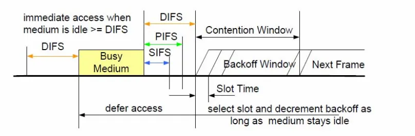
In the MAC layer, two channel access functions are specified in the standard. The mandatory contention-based channel access function is called the DCF (Distributed Coordination Function) which is based on the CSMA/CA (Carrier Sense Multiple Access with Collision Avoidance), Figure 2.2 shows Basic channel access mechanism of IEEE 802.11 DCF.

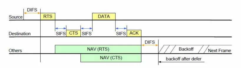
Most IEEE 802.11 WLAN devices use the DCF for shared wireless channel access. In the DCF, when multiple frames are transmitted simultaneously by different stations, a collision occurs, which destroys most of all the transmitted frames. To resolve collisions, the stations employ a binary slotted exponential back-off algorithm and retransmission scheme. Moreover, the IEEE 802.11 provides a MAC layer data acknowledgment to recover the frame losses due to the channel error and the channel reservation mechanism to reduce the collision probability. With the 4-way handshake mechanism, before a data frame is sent, the station senses the channel conditions. If the channel is idle for at least a DIFS (DCF Inter-Frame Space) period of time, a sender starts its transmission request by sending a RTS (Request To Send) frame to the receiver. The receiver, after a time called SIFS (Short Inter Frame Space), replies with a CTS (Clear To Send) frame. All stations hearing RTS and CTS (i.e. the stations in the sender and receiver radio range) set the NAV (Network Allocation Vector) to the time necessary to complete the data frame transmission in order to defer their transmissions during this time. When the sender receives a CTS frame, it waits for the SIFS and transmits the data frame. After receiving the data frame correctly, the receiver waits for the SIFS and sends an ACK frame [1]; Figure 2.3 shows RTS/CTS exchange mechanism of IEEE 802.11.

  11

2.1.2 Physical Layer

Physical layer (PHY) is the interface between the MAC layer and the wireless medium. It transmits and receives DATA frames over the shared wireless medium. The frame exchange between MAC and PHY is controlled by the Physical Layer Convergence Procedure (PLCP) sublayer. Employing different modulation and channel coding schemes enables the 802.11 PHY to provide multiple transmission rates.

2.2 Rate Adaptation Schemes

The IEEE 802.11 PHY provides multiple data transmission modes. A higher data rate does not necessarily yield a higher throughput. Only when the channel conditions are good, does a higher data rate give a higher throughput. To accommodate different wireless channel conditions, due to fading, interference, and mobility, and so on, the rate adaptation scheme is commonly employed. This is realized by dynamically adjusting the modulation and coding levels to optimize performance over time-variant wireless channel conditions. Since the IEEE 802.11 standard does not specify any mechanism and protocol to efficiently utilize the multiple data transmission rates, many rate adaptation schemes have been proposed and some have been used in real products. The basic idea of these schemes is to estimate the channel quality and adjust the data transmission mode accordingly. This is typically achieved by using a few metrics collected at the sender and the associated design rules. The widely used metrics include probe packets, consecutive successes or losses, PHY metrics such as SNR (Signal to Noise Ratio) or SSI (Signal Strength Indicator), and long-term statistics [8].

  13 Among the existing statistics-based rate adaptation schemes, the earliest and the most widely used one is ARF (Auto Rate Fallback), which was used in Lucent’s WaveLAN-II product [11]. In the ARF scheme, a discrete set of data rates are used. If the ACK frames for two consecutive data frames "m" are not received by the sender, then the sender drops the transmission rate to the next lower data rate and a timer is started. If ten consecutive data frames "n" are successfully received or the timer expires, then the transmission rate is raised to the next higher data rate and the timer is stopped. When the rate is increased, the first transmission must be successful or the rate is immediately decreased and the timer is started again. Specifically, the value of m and n is 2 and 10 respectively adopted by Lucent Technologies' Wave LAN-II products [11]. Lacage et al. proposed the AARF (Adaptive ARF) which continuously adjusts the interval of the transmission rate changes at runtime [3]. Many commercial WLAN products have implemented ARF or similar schemes based on the same concept. Despite the wide applicability of ARF scheme, this scheme can be dysfunctional when multiple stations coexist. When there are a number of stations that can hear each other, and the ARF scheme is enabled in all the stations in a WLAN, these stations may misinterpret frequent collisions as channel error losses and accordingly reduce their data transmission rate unnecessarily. To overcome the collision problem in the ARF scheme, the CARA (Collision-Aware Rate Adaptation) scheme has been proposed. The key concept of the CARA scheme is that the sender combines adaptively the RTS/CTS exchange with the CCA (Clear Channel Assessment) functionality to differentiate collisions from frame transmission failures caused by channel errors. Therefore compared with other statistics-based rate adaptation schemes, the CARA scheme decides the data transmission mode more precisely and improves the wireless link utilization [4]. However, a fundamental limitation of statistics-based approaches is that they classify channel conditions as either ”good” or ”bad”. This binary decision provides some notion about the direction in which to adapt the transmission mode, but does not suffice to select the appropriate mode immediately. This leads to a slow step-by-step accommodation to large changes in channel conditions, and introduces the risk of oscillation in a stable channel conditions.

example is the RBAR (Receiver-Based Auto Rate) scheme [13] which performs rate adaptation at the receiver instead of at the sender. The RBAR mandates the use of RTS/CTS exchange. The receiver of an RTS frame calculates the transmission rate to be used by the sender based on the measured SNR from the received RTS frame and on a set of SNR thresholds calculated with an a priori wireless channel model. Knowing the current SNR and the throughput-vs.-SNR curves for each transmission rate solves how to select the data transmission mode. It simply selects to the transmission mode with the highest throughput for the current SNR. The rate to be used to send the data frame is then returned to the sender in the CTS frame. The RTS, CTS and data frames are modified to deliver more information on the size and the data transmission rate to allow all the stations within the transmission range to correctly update their NAV.

Despite the advantages, SNR based rate adaptations have not been applied in practice so far. This is mainly because of three reasons. First, the RTS/CTS channel access procedure is required even if no hidden terminals are present. The extra overhead incurred by an RTS/CTS exchange is well known. Secondly, it requires the receivers to measure SNR, which may be difficult to realize in low cost WLAN devices. Finally, it is incompatible with the IEEE 802.11 standards because of the edified RTS/CTS frames format and the RSH (Reservation Sub Header).

  15

Figure 2.4. Classification of existing algorithms as an open loop algorithm or a close loop algorithm

2.3 Artificial Neural Network

2.3.1 Introduction to Artificial Neural Network

A Neural Network is a powerful data-modeling tool that is able to capture and represent complex input/output relationships. The motivation for the development of neural network technology stemmed from the desire to develop an artificial system that could perform "intelligent" tasks similar to those performed by the human brain. Neural networks resemble the human brain in the following two ways:

• A neural network acquires knowledge through learning.

An artificial neural network is a massively parallel distributed processor made up of simple processing units (neurons), which has the ability to learn functional dependencies from data.

2.3.2 Advantages of neural networks

• Adaptive learning: An ability to learn how to do tasks based on the data given for training or initial experience.

• Self-Organization: An ANN can create its own organization or representation of the information it receives during learning time.

• Real Time Operation: ANN computations may be carried out in parallel, and special hardware devices are being designed and manufactured which take advantage of this capability.

• Fault Tolerance via Redundant Information Coding: Partial destruction of a network leads to the corresponding degradation of performance. However, some network capabilities may be retained even with major network damage [16].

The procedure used to perform the learning process is called a learning algorithm, the function of which is to modify the synaptic weights of the network in an orderly fashion to attain a desired design objective.

Each neuron is a simple processing unit which receives some weighted data, sums them with a bias and calculates an output to be passed on the function that the neuron uses to calculate the output is called the activation function. Typically, activation functions are generally non-linear having a "squashing" effect. Linear functions are limited because the output is simply proportional to the input.

  17 in one layer is connected to every perceptron on the next layer; hence information is constantly "fed forward" from one layer to the next.

By varying the number of nodes in the hidden layer, the number of layers, and the number of input and output nodes, one can classify points in arbitrary dimensional space into an arbitrary number of groups.

2.3.3 Neuron model

The multilayer perception neural network is designed from simple components. Initially, we will describe a single input neuron which is then extended to include multiple inputs. Next, these neurons will be stack together to produce a layer [15]. Finally, a number of layers are cascaded together thus forming a multilayer network.

2.3.3.1 Single-input neuron

A single-input neuron is shown in figure 2.5. The scalar input p is multiplied by the scalar weight "W" to form "Wp", one of the terms that are sent to the summer. The other input, "1", is multiplied by a bias "b" and then passed to the summer. The summer output "n" often referred to as the net input, goes into a transfer function "f" which produces the scalar neuron output (sometimes "activation function" is used rather than transfer function and offset rather than bias).

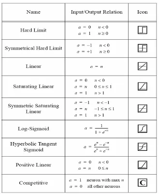
From Figure 2.5, both "w" and "b" are both adjustable scalar parameters of the neuron. Typically the transfer function is chosen by the designer and then the parameters "w" and "b" will be adjusted by some learning rule so that the neuron input/output relationship meet some specific goal. The transfer function in Figure 2.5 may be a linear or nonlinear function of n. A particular transfer function is chosen to satisfy some specification of the problem that the neuron is attempting to solve. Figure 2.6 shows some common transfer functions.

  19

2.3.3.2 Multiple-input neuron

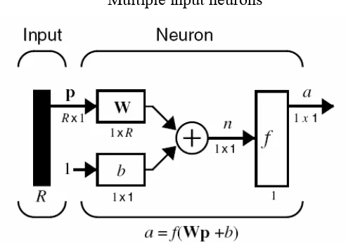
Typically, a neuron has more than one input. A neuron with R inputs is shown in figure 2.7. The individual inputs p , p_{1 2}…p _g are each weighted by corresponding elements of the weight matrix "W". The neuron has a bias "b", which is summed with the weight inputs to form the net input "n":

1,1 1,2 1,R W W , .W …

1,1 1 1,2 2 1,R R

n =W p +W p +... +W p + b (1)

This expression can be written in matrix form as:

n = Wp + b (2)

Figure 2.7: Multiple-input neuron.

A particular convention in assigning the indices of the elements of the weight matrix has been adopted [15]. The first index indicates the particular neuron destination for the weight. The second index indicates the source of the signal fed to the neuron. Thus, the indices in " " say that this weight represents the connection to the first (and only) neuron from the second source [15]. A multiple-input neuron using abbreviated notation is shown in Figure 2.8.

Multiple input neurons

Figure 2.8: A multiple-input neuron using abbreviated notation.

As shown in figure 2.8, the input vector "p" is represented by the solid vertical bar at left. The dimensions of "p" are displayed below the variable as "Rx1", indicating that the input is a single vector of "R" elements. These inputs go to the weight matrix "W", which has "R" columns but only one row in this single neuron case.

A constant "1" enters the neuron as an input and is multiplied by a scalar bias "b". The net input to the transfer function "f" is "n", which is the sum of the bias "b" and the product "Wp". The neuron's output is a scalar in this case. If there exit more than one neuron, the network output would be a vector.

2.3.3 Multilayer perceptron network architectures

  21

2.3.3.1 A layer of neurons

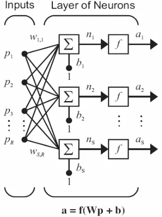
A single-layer network of "S" neurons is shown in figure 2.9. Note that each of the "R" inputs is connected to each of the neurons and that the weight matrix now has s rows.

Figure 2.9: A single-layer network of S neurons.

The layer includes the weight matrix, the summers, the bias vector

" "

_"

b

p" is connected to each neuron through the weight matrix "W". Each neuron has a bias b , _i a summer, a transfer function f and an output " ". Taken together, the outputs form the output vector "a

"

i

a

≠S). The input vector elements enter the network through the weight matrix "W":

1,1 1, ,1 , R S S w w w

w w R

⎡ ⎤ ⎢ ⎥ = ⎢ ⎥ ⎢ ⎥ ⎣ ⎦ L

M O M

K

The row indices of the elements of matrix "W" indicate the destination neuron associated with that weight, while the column indices indicate the source of the input for that weight. Thus, the indices in " " say that this weight represents the connection to the third neuron from the second source. The S-neuron, R-input, one-layer network also can be drawn in abbreviated notation as shown in Figure 2.10.

3,2 W

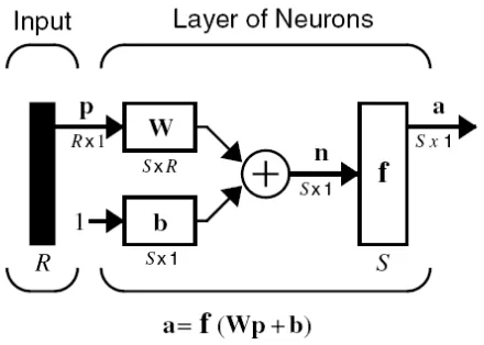
Figure 2.10: Layer of S neurons, abbreviated notation

Here again, the symbols below the variables tell that for this layer, "p" is a vector of length "R", "W" is an "S*R" matrix and

_"

"

"

defined previously, the layer includes the weight matrix, the summation and multiplication operations, the bias vector

_"

"

vector.

a

2.3.3.2 Multilayer perceptron (MLP)

Considering a network with several layers, each layer has its own weight matrix "W", it’s own bias vector "b", a net input vector "n" and an output vector " ". Some additional notation should be introduced to distinguish between these layers. Superscripts are used to identify these layers. The number of the layer as a superscript is appended to the names for each of these variables. Thus, the weight matrix for the

  23

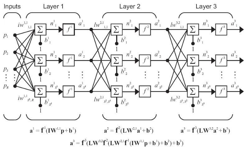
second layer is written as . This notation is used in the two-layer network shown in Figure 2.11.

2 w

There are "R" inputs, " " neurons in the first layer, " " neurons in the second layer, etc. The output of layers one and two are the inputs for layers two and three. Thus layer 2 can be viewed as a one-layer network with R= inputs, S= neurons and an * weight matrix . The input to layer 2 is and the output is . A layer whose output is the network output is called an output layer. The other layers are called hidden layers.

1

S 2

S

1

S _S2

1

S _S2 _W2 1

a a2

Figure 2.11. Three layer network

Figure 2.12: abbreviated notation of multilayer network

The network learns about the input through an interactive process of adjusting the weights and the bias. This process is called supervised learning and the algorithm used is the learning algorithm. One of the most common is the error back propagation algorithm. This algorithm is based on the error-correction learning rule, based on gradient descent in the error surface.

  54

REFERENCES

[1] IEEE Std 802.11-1999, “Wireless LAN medium access control (MAC) and physical layer (PHY) specifications,” Jun. 2003.

[2] IEEE 802.11 a/b, Wireless LAN Medium Access Control (MAC) and Physical Layer (PHY) Specifications, Standard, IEEE, Aug. 1999.

[3] M. Lacage, M.H. Manshaei, and T. Turletti. "IEEE 802.11 rate adaptation: a practical approach." Proceedings oj'the 7th ACM international symposium on modeling, analysis and simulation of Wireless and mobile systems, pages 126- 134,2004.

[4] J. Kim, S. Kim, S. Choi, and D. Qiao. "CARA: Collision Aware Rate Adaptation for IEEE 802.11 WLANs." IEEE INFOCOM, 2006.

[5] F. Maguolo, M. Lacage, T. Turletti. "Efficient Collision Detection for Auto Rate Fallback Algorithm." IEEE INFOCOM, 2008.

[6] P. Kulkarni, S. Quadri. "Simple and Practical Rate Adaptation Algorithms for Wireless Networks." IEEE INFOCOM, 2009.

[7] S. Khan, S. A. Mahmud, K. K. Loo, and H. S. AI-Raweshidy, "A Cross Layer Rate Adaptation Solution for IEEE 802.11 Networks," Computer Communications, Vol. 31, Issue 8, May 2008, pp. 1638 - 1652.

[8] S. H. Y. Wong, H. Yang, S. Lu, and V. Bharghavan, "Robust Rate Adaptation for 802.11 Wireless Networks," in Proc. oj' ACM MOBICOM 2006, pp. 146 - 157.

[9] M. Heusse, F. Rousseau, G. Berger-Sabbatel, and A. Duda, "Performance Anomaly of 802.11b ," in Proc. oj'lEEE INFOCOM 2003, pp. 836 - 843.

[10]IEEE 802.llg Part II, Wireless LAN Medium Access Control (MAC) and Physical Layer (PHY) Specifications, IEEE, 2003.

[11]A. Kamerman and L. Monteban, "WaveLAN-II: A High-Performance Wireless LAN for The Unlicensed Band," Bell labs Technical J., summer 1997, pp. 118 – 133.

[12]I. Haratcherev, J. Taal, K. Langendoen, R. Lagendijk, and H. Sips, "Automatic IEEE 802.11 rate control for streaming applications," Wireless Communications and Mobile Computing, 2005.

[13]G. Holland, N. Vaidya, and P. Bahl, "A rate-adaptive MAC protocol for multi-hop wireless networks," ACM/IEEE MOBICOM, pp.236-250, 2001.

[14]F. Maguolo, M. Lacage, T. Turletti. "Efficient Collision Detection for Auto Rate Fallback Algorithm." IEEE INFOCOM, 2008.

[15]S. Haykin, "Neural Networks: A Comprehensive Foundation," 2nd edition, Prentice Hall.

[16]Christos Stergiou and Dimitrios Siganos, “Neural Networks”, Computer Science Deptt. University of U.K., Journal, Vol. 4, 1996.

[17]Walter, H. Delashmit and Michael T. Manry, 2005. Recent Developments in Multilayer Perceptron Neural Networks. Proceedings of the 7th Annual Memphis Area Engineering and Science Conference, MAESC 2005.