High Resolution Spectral Estimation using BP via
Compressive Sensing
Isabel M. P. Duarte, Jos´e M. N. Vieira, Paulo J. S. G. Ferreira, and Daniel F. Albuquerque
Abstract—In this paper we propose a method based on compressed sensing (CS) for estimating the spectrum of a signal written as a linear combination of a small number of sinusoids. In the case of finite-length signals, the Fourier coefficients are not exactly sparse due to the leakage effect if the frequency is not a multiple of the fundamental frequency; To overcome this problem our algorithm transform the DFT basis into a frame with a larger number of vectors, by inserting columns between some of the initial ones. The algorithm applies Basis Pursuit (BP) to estimate the sinusoids amplitude, phase and frequency.
Index Terms—Basis Pursuit, compressive sensing, spectral estimation, sparse representations.
I. INTRODUCTION
T
HE compressive sensing theory allows us to recover,sparse or compressible signals, from a number of
mea-surementsM, much smaller than the lengthN of the signal.
Instead of acquiring N samples, compute all the transform
coefficients and then discard the small ones, we can acquire
a number of random mixtures proportional to the sparsityK.
The samples are obtained projecting x on a set of M
vectors{ϕi} ∈RN, that are independent of the signal, with
which we can build the sampling matrix Φ∈RM×N, with
M < N. The measurement vector is obtained byy= Φx.
To reconstruct the K-sparse signal x, we search for the
sparsest coefficient vector x, solving the underdetermined
systemy= Φx. Since the matrixΦis rank deficient, and so
it loses information, one can think the problem is impossible, but it can be shown that if the matrix obeys the Restricted
Isometry Property (RIP), we can recoverxexactly by solving
the convex problem [1], [2]:
(P1) : min∥x∥1:y= Φx, (1)
where∥x∥1= Σ|xi|.
Essentially, the RIP requires that every set of less thanK
columns, approximately behaves like an orthonormal system. More precisely, let ΦT, T ⊂ {1,· · · , N}, be the M × |T|
submatrix consisting of the columns indexed by T. TheK
-restricted isometry constantδK ofΦis the smallest quantity
such that
(1−δK)∥x∥2≤ ∥ΦTx∥2≤(1 +δK)∥x∥2 (2)
for all the subset T ⊂ N, with |T| ≤ K and coefficient
sequences(xj), j∈T.
The signal x, which isK-sparse or compressible, can be
recovered by solving the indeterminate system y = Φx, by
Manuscript received July 18, 2012; revised August 09, 2012.
Isabel M. P. Duarte, School of Technology and Management of Viseu, Polytechnic Institute of Viseu and Signal Processing Lab., IEETA/DETI, University of Aveiro, e-mail:[email protected]
Jos´e M. N. Vieira, Paulo J. S. G. Ferreira, Daniel F. Albuquerque, Signal Processing Lab., IEETA/DETI, University of Aveiro
(P1), from only M ≥CKlog(N/K) samples, particularly
with matricesΦ, with Gaussian entries [3].
The problem (P1) cannot be solved analytically, but can be reformulated as a linear programming problem when the data is real, and as a second order cone problem when
the data is complex [4], [5]. In the complex case, ∥x∥1
is neither a linear nor a quadratic function of the real and imaginary components, and cannot be reformulated as one:
∥x∥1 =
∑ √
ℜ(xi)2+ℑ(xi)2. In this case, the problem
can be reformulated into second order cone programming,
(SOCP), and solved with algorithms implemented in the framework of Interior Point Methods, for example using the
CVX algorithm [6]. If a signal xcan be written as a linear
combination of K sinusoids, the signal presents few
non-zero spectral lines in the classical Fourier Transform sense,
that is, it is K-sparse in the frequency domain. However,
in practical applications, because we use finite N-length
signals, the signal is sparse only if the frequencies are
mul-tiples of the fundamental frequency 2Nπ. Leakage limits the
success of the traditional CS algorithms. Here, we propose an iterative algorithm which find a first approximate location of a sinusoid and then refine the sampling in frequency around the neighborhood of this sinusoid up to a required precision. If several sinusoids have to be found, the procedure iterate as many times as needed this locale refinement.
The idea comes from the dual problem of fractional time-delay estimation, as studied in the work of Fuchs and Deylon [7]: the true value of the frequency can be obtained by BP between frequencies values having the higher values.
II. SPECTRALESTIMATIONWITHCOMPRESSIVE
SENSING
Consider Ψ∈ CN×N as the inverse of the DFT matrix.
Then, if xis a time domain discrete signal with length N,
the DFT of x will be s = Ψ−1x. If x is observed using
random measurements, we havey = Φx, and we can write
the problem (P1), from the equation (1):
min∥s∥1:y= ΦΨs= Θs, (3)
The CS theory ensures that a signal that is sparse or
compressible in the basis Ψ can be reconstructed from
M = O(Klog(NK)) linear projections onto a basis Φ that
is incoherent with the first, solving the problem (P1) using the equation (3), [8], [9].
Ifxcontains only sinusoids with frequencies multiples of
2π
N rad, thens will be a sparse signal. Otherwise,s will be
not sparse. If we apply the CS to solve this problem, the
recovered signals will not be sparse, as we can see in the
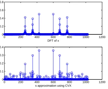
example depicted in Fig. (1). The error is0.5986and even if
we increase the number of measurements, the error remains
0.2892for M = 150. Since the signal is not sparse we will need more measurements to get a better result. This comes
0 200 400 600 800 1000 1200 0
0.2 0.4 0.6 0.8
DFT of x
0 200 400 600 800 1000 1200 0
0.1 0.2 0.3 0.4
[image:2.595.87.264.99.244.2]s approximation using CVX
Fig. 1. Spectrum of a signal with lengthN = 1024composed of three sinusoids that are not multiple of the fundamental frequency of the DFT, using the DFT and the CS usingM= 50measurements.
from the fact that no column vector in the matrix Ψ has
a frequency matching one of the frequencies present in the
signal. The first idea is to expand the matrixΨ, so that each
frequency present in the signal is represented by a column. We would have a redundant frame instead of the orthogonal basis of the DFT. By increasing the frame size, signals with frequencies that are not multiples of the fundamental frequency of the DFT become more compressible, resulting into a recovery performance improvement, but in return, the frame becomes increasingly coherent, which leads to a decrease in performance recovery. So the idea was to add only a small number of columns. If we know between which
columns of the Ψ matrix, are the frequencies that are not
multiples of the fundamental frequency, we can add columns
to the matrixΨ, only in that interval, but in CS we only have
access to the signal y.
A. Problem of fractional time-delay estimation
The dual problem of the fractional frequency spectral estimate is the fractional time-delay estimation. Fuchs and Deylon, in [7], presented an analytical expression of the
minimalℓ1-norm interpolation function which is independent
of the signal, to solve the problem to get an estimate of the
delay τ, having a bandlimited signal x(t), with a maximal
sampling period h= 1, which is given byy(t) =x(t−τ).
One possibility is to seek the valuessn in
y(t) =x(t−τ) =∑
n
x(t−nh)sn.
An estimation of the delay τ is determined from the
max-imum location of the interpolating function which is given by
ψ(t) =∑
k≥0
βkϕ(|t| −k)
|t| , |t| ∈[k, k+
1
l],
with
ϕ(x) = 1
Γ(x)Γ(1l −x), x∈[0,
1
l],
βk = (−1)kΓ(k+
1
l)
Γ(k+ 1),
whereΓis the standard gamma function. This reconstruction
function is very localised and as the oversampling factor,l,
increases more localised it will be, unlike what happens with the sinc function, which keeps the width of the main lobe, as one can see in Fig. (2).
−3 −2 −1 0 1 2 3
−0.5 0 0.5 1
Graphic using l= 2
−3 −2 −1 0 1 2 3
−0.5 0 0.5 1
Graphic using l= 5
interp. function sinc function
[image:2.595.326.517.126.278.2]interp. function sinc function
Fig. 2. ℓ1-norm interpolating function with oversampling factorsl= 2
andl= 5, compared with the sinc function.
Since the minimal ℓ1- norm reconstruction function is
quite localised, the sn values can be obtained by solving
the minimalℓ1-norm problem
min∥sn∥1:y(t) =
∑
n
x(t−nh)sn, h <1,
which is the BP.
The problem we are dealing with is the dual of the problem studied by these authors. If we have a signal with a frequency
fi, which is a multiple of the fundamental frequency of the
DFT, we know that the DFT of the signal has a maximum in the position of this frequency.
Looking to the frequency of the signal as the dual of the delay, the interpolating function will have a maximum exactly in the same place, independently of the considered
l value. If we have a signal with a frequencyfi, which is
not multiple of the DFT fundamental frequency, the signal is not sparse, therefore there are no maximums. However, the interpolating function will have a maximum in the position
of the frequency, regardless of the amount of l which is
considered. If the signal has two frequencies that are not multiples of the fundamental frequency, the interpolating function has two maximums, both between the values of the frequencies with higher values obtained by BP. See the example depicted in Fig. (3).
Thus, one possible solution to our problem of knowing where the frequencies are, is to apply the BP. Each of the frequencies in question, will be between the position of the two frequencies multiple of the fundamental frequency, where BP obtains maximum values.
If the frequencies are very close, a greater value oflmust
be used in order to discover them. See Fig. (4).
0 1 2 3 4 5 6 7 −0.1
0 0.1 0.2 0.3 0.4 0.5 0.6
Frequencies (rad)
With l= 2 and frequencies 7.2*2pi/32 and 7.6*2pi/32
BP
[image:3.595.69.263.49.209.2]interpolating function
Fig. 3. Minimall1norm using BP and using thel1interpolating function.
0 0.5 1 1.5 2 2.5 3
0 0.2 0.4 0.6 0.8
frequencies (rad)
With l= 2 and frequencies 7.2*2pi/32 and 7.6*2pi/32
BP
interpolating function
0 0.5 1 1.5 2 2.5 3
0 0.2 0.4 0.6 0.8
frequencies (rad)
With l= 9 and frequencies 7.2*2pi/32 and 7.6*2pi/32
BP
[image:3.595.73.260.234.393.2]interpolating function
Fig. 4. Minimall1 norm using BP and using the interpolating function
with frequencies very close, using two values ofl.
Therefore, to determine the approximated value of another frequency, we expand the original matrix by adding that column. Then, by applying again the BP we find another interval and we repeat the same procedure.
This algorithm can be easily extended for more frequencies as shown in the next section.
B. Algorithm
We begin by calculatingˆs, which is the approximate value
of s, solving the minimisationℓ1-norm problem:
ℓ1: min∥s∥1:y= Θs.
Then:
1) We will calculate the argmax ofsˆ,smax;
2) The interval [smax−1, smax] or [smax, smax+ 1] is
chosen as the image nearest to smax. Let’s call this
interval [a,b];
3) We will add columns between the two extremes that correspond to the interval considered in the previous point:
I:= 0
while (I <Nmaxpoint andϵ >error threshold)
a) I:=I+ 1
b) We will consider matrix Ψ1, adding I columns
to Ψ. The I frequencies of columns to add are
given by:(a+ (1 :I)/(I+ 1))−1.
c) We will calculate the ˆs values, in the interval
[a, b], considering the matrix Ψ1;
d) We will calculate the argmax ofsˆ, only in the in-terval[a, b], which contain theI added columns;
e) We will consider a new matrix, Ψ2, from Ψ,
where in the interval [a, b] is added the column
which corresponds to the argmax of the values obtained in the previous point;
f) We will calculate the sˆvalues, using the matrix
Ψ2;
g) We compute the value of ϵ
4) Ψ = Ψ2
5) We will repeat the steps from 1. to 4. as many times as the sparsity of the signal.
In the end we calculate the valuexˆ= Ψˆs.
In this algorithm, we use the standard error, given by
erro= ∥x∥−x∥xˆ∥. The stopping criterion in the reconstruction of the approximate value for each frequency,ϵ, i.e, the criteria
used to stop adding columns in the range [a, b]is given by
the difference between the errors obtained in two consecutive iterations. In each iteration the error is given by the sum of
absolute values ofˆsexcluding theKhigher values, with K
the value of sparsity. If in the interval[a, b], on the step 3f., we add the column corresponding to the frequency of the sinusoid, this error is very small.
III. EXPERIMENTALRESULTS
In our experiments we use signals of length N = 1024
samples and all the signals contain real-value sinusoids, with random frequencies. The amplitudes of each frequency is 1 except in the experiment III.
A. Experiment I
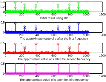
In our first experiment, we apply the proposed algorithm to
a signal containing three real-value sinusoids,K= 6, using
M = 100 measurements. Therefore we can reconstruct the
signal with an error of 0.0268, which had an initial error of 0.5275, see Fig. (5).
0 200 400 600 800 1000 1200 0
0.2 0.4
Initial result using BP
0 200 400 600 800 1000 1200 0
0.5
The approximate value of s after the first frequency
0 200 400 600 800 1000 1200 0
0.5
The approximate value of s after the second frequency
0 200 400 600 800 1000 1200 0
0.5
The approximate value of s after the third frequency
Fig. 5. The approximate value ofs, first using CVX to solve the BP, and then with the proposed algorithm in the first, second and third frequencies.
As shown in Fig. (6), the error decreases exponentially as we add columns in the interval, so we can initialise the number of adding columns, step 1. of the proposed algorithm,
with a greater value than I = 1. In our experiments we
[image:3.595.337.515.544.682.2]0 500 1000 1500 10−4
10−3 10−2 10−1 100
Number of added columns (I)
[image:4.595.339.514.55.377.2]Error between iterations I and I−1
Fig. 6. The error in the first frequency in function of the number of added columns.
50 100 150 200 250 300 350 400 10−5
10−4 10−3 10−2 10−1 100
Number of measurements, M
Error
[image:4.595.70.263.64.219.2]1f 2f 3f
Fig. 7. Performance of CS signal recovery with the proposed algorithm for signals with one, two, three and four frequencies which correspond to
K= 2,K= 4andK= 6respectively. All quantities are averaged over 400 independent trials.
B. Experiment II
Our second experiment compares the performance of the proposed algorithm for signals with one, two and three frequencies. We verify that the number of measurements we need for the same performance increases with the sparseness of the signal. See Fig. (7).
C. Experiment III
This experiment shows the behaviour of the proposed algorithm, when the amplitudes of the signal frequencies are different. Fig. (8) presents the result of the signal re-covery using our algorithm for a signal composed by three random frequencies with amplitudes 1, 0.01 and 0.05. The proposed algorithm performs better for different amplitudes, than Thresholding based algorithms, like Spectral Iterative
Hard Thresholding (SIHT) proposed by M. Duarte andet al.
in [10], since the Thresholding algorithms consider, in each
iteration, only theK largest spectral components, removing
the others. With this approach, the smallest frequencies can be discarded.
D. Experiment IV
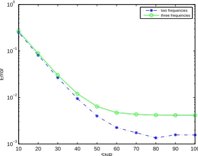
Our fourth experiment tests the robustness of the proposed algorithm to additive noise in the measurements of a signal
0 200 400 600 800 1000 1200 0
0.05 0.1 0.15 0.2 0.25 0.3 0.35 0.4 0.45 0.5
The approximated value of s
f=417.1386*2pi/N; amp=1, f=65.0176*2pi/N; amp=0.01 e f=463.7652*2pi/N; amp=0.05
(a)
0 200 400 600 800 1000 1200
10−12 10−10
10−8
10−6
10−4 10−2 100
The approximated value of s
f=417.1386*2pi/N; amp=1, f=65.0176*2pi/N; amp=0.01 e f=463.7652*2pi/N; amp=0.05
[image:4.595.65.261.261.414.2](b)
Fig. 8. The approximate value s, for a signal containing three real-value sinusoids with frequencies of amplitudes 1, 0.01 and 0.05
written as a linear combination of two and three sinusoids. The error was evaluated for ten signal to noise ratios (SNR) and the results are depicted in Fig. (9). As we can see, the proposed algorithm performs quite well.
10 20 30 40 50 60 70 80 90 100 10−3
10−2 10−1 100
SNR
Error
two frequencies three frequencies
Fig. 9. Performance of signal recovery using the proposed algorithm for a signal composed by two and three different frequencies with 150 noisy measurements. All quantities are averaged over 100 independent trials.
E. Experiment V
This experiment compares the performance of the pro-posed algorithm with two of the algorithms propro-posed by M.
Duarte andet al.in [10], which they called by Spectral CS
[image:4.595.322.518.486.640.2]For the SIHT, the authors use an over-sampled DFT frame and a coherent-inhibiting structured signal model, that inhibits closely spaced sinusoids, and the classical sinusoid parameter estimation algorithm, periodogram. In our algo-rithm we do not need to impose a model based, to inhibit the coherence of the frame, because our interpolating function is very localised.
50 100 150 200 250 300 350 400 450 500 10−4
10−3 10−2 10−1 100
Number of measurements, M
Error
[image:5.595.322.522.98.355.2]Proposed algorithm SIHT via Periodogram music
Fig. 10. Performance of signal recovery using the proposed algorithm, using the SIHT implemented via heuristic algorithm and using the Root Music algorithm. All quantities are averaged over 400 independent trials.
F. Experiment VI
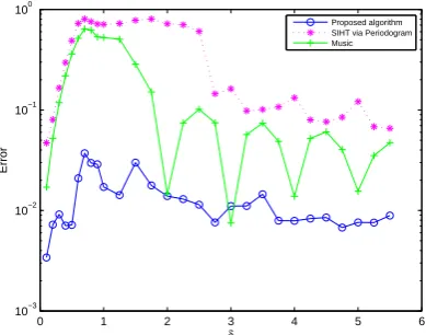
Our last experiment shows how the proposed algorithm behaves for two close frequencies and compares its perfor-mance with the perforperfor-mance of the SIHT and the Root Music
algorithms. We have considered a fixed frequency,f1 and a
second frequency, f2 = f1+δ, where δ = [0.1 : 0.1 :
1,1.25 : 0.25 : 5.5]. As shown in Fig. (11), our algorithm
presents a better performance than the others.
0 1 2 3 4 5 6
10−3 10−2 10−1 100
δ
Error
[image:5.595.66.260.154.301.2]Proposed algorithm SIHT via Periodogram Music
Fig. 11. Performance of signal recovery using the proposed algorithm, the SIHT implemented via heuristic algorithm and the Root Music algorithm, considering a signal with two frequencies where f2 = f1+δ. We have
used 100 measurements. All quantities are averaged over 200 independent trials.
Note that, although the errors are small for delta values smaller than 1, the frequencies values can be very different from the correct ones, as we can see in TABLE I
The results of the proposed algorithm were as it was
expected, since the minimal ℓ1-norm interpolation function
is very localised, unlike the minimal ℓ2-norm interpolation
function - the sinc function, as one can see in Fig. (12).
TABLE I
RECOVERED VALUES OBTAINED WITH THE PROPOSED ALGORITHM,THE
ROOTMUSIC ALGORITHM AND THE SIHT ALGORITHM,USING THE FIXED FREQUENCYf1ANDf2=f1+δ.
Frequencies Prop. Algorithm MUSIC SIHT
δ δδ
δ ࢌ ࢌ ࢌ ࢌ ࢌ ࢌ ࢌ ࢌ 0.1000 463.7655 463.8655 463.7638 464.8000 78.8620 463.8151 0.0000 0.0000
0.2000 463.7655 463.9655 463.7621 464.8000 52.4859 463.8594 460.4439 463.8723
0.3000 463.7655 464.0655 464.0734 464.0000 265.7705 463.9192 460.4508 463.9125
0.4000 463.7655 464.1655 463.8000 464.2148 67.0411 463.9667 22.8131 463.9436
0.5000 463.7655 464.2655 464.2000 463.7007 464.0346 469.9109 378.3570 463.8356 0.6000 463.7655 464.3655 463.9000 464.4437 0.0377 397.5788 459.2702 463.8318
0.7000 463.7655 464.4655 463.4965 464.5676 370.1165 464.2669 246.8810 463.3999
0.8000 463.7655 464.5655 464.6005 463.7246 212.0844 463.8000 129.2858 464.9987
0.9000 463.7655 464.6655 464.6176 463.7699 408.0093 463.6348 255.1839 463.5699
1.0000 463.7655 464.7655 463.5866 464.8085 406.0506 464.8486 199.8234 464.9885
0 0.5 1 1.5 2 2.5 3
−0.1 0 0.1 0.2 0.3 0.4 0.5 0.6 0.7 0.8
Graphic using l= 9
9 pts DFT BP
interpolating function
Fig. 12. Minimalℓ1-norm using BP and using the interpolating function
with an over sampling factor ofl = 9. The dotted curve is the minimal
ℓ2-norm interpolating function: the sinc function.
IV. CONCLUSION
We have developed a new algorithm to estimate the spec-tral components in the case of sparse finite-length signals. The algorithm uses a redundant frame, transforming the DFT basis into a frame with a larger number of vectors, by inserting columns between some of the initial ones.
From the results can be seen that the proposed algorithm can recover the sparse signals with an error smaller than
0.001, even for a signal withK= 6.
Furthermore, it presents a good performance in the pres-ence of noise. In addition to this, it can deal with sig-nals where the frequency amplitudes are very different, overcoming other algorithms in this field. Moreover, the proposed algorithm performs better than others that we have compared for the same signal while using the same number of measurements.
ACKNOWLEDGMENT
The authors would like to thank to Polytechnic Institute of Viseu and to IEETA - University of Aveiro.
REFERENCES
[1] D. Donoho and X. Huo, “Uncertainty principles and ideal atomic decomposition,”IEEE Transactions on Information Theory, vol. 47, no. 7, pp. 2845 – 2862, 2001.
[2] E. J. Cands, J. K. Romberg, and T. Tao, “Stable signal recovery from incomplete and inaccurate measurements,”Communications on Pure and Applied Mathematics, vol. 59, no. 8, pp. 1207–1223, 2006. [3] J. Tropp and A. Gilbert, “Signal recovery from random measurements
[image:5.595.65.260.484.637.2][4] D. M. Malioutov, “A sparse signal reconstruction perspective for source localization with sensor arrays,” Master’s thesis, MIT, July 2003.
[5] S. W. Makino, H. Sawada, and Shoji, “On real and complex valued L1-norm minimization for overcomplete blind source separation,” pp. 86 – 89, 2005.
[6] M. G. Boyd and S., “Matlab software for disciplined convex program-ming, version 1.21,” 2011.
[7] J. J. Fuchs and B. Delyon, “Minimal L1-norm reconstruction function for oversampled signals: applications to time-delay estimation,”IEEE Transactions on Information Theory, vol. 46, no. 4, pp. 1666–1673, 2000, journal.
[8] D. Donoho, “Compressed sensing,”IEEE Transactions on Information Theory, vol. 52, no. 4, pp. 1289 – 1306, 2006.
[9] E. Candes, J. Romberg, and T. Tao, “Robust uncertainty principles: exact signal reconstruction from highly incomplete frequency infor-mation,”IEEE Transactions on Information Theory, vol. 52, no. 2, pp. 489– 509, 2006.
[10] R. G. Baraniuk and M. F. Duarte, “Spectral compressive sensing,”