A Simple and Effective Method for Injecting Word Level Information into Character Aware Neural Language Models

Proceedings of the 23rd Conference on Computational Natural Language Learning, pages 920–928 920

A Simple and Effective Method for Injecting Word-level Information into

Character-aware Neural Language Models

Yukun Feng1, Hidetaka Kamigaito1, Hiroya Takamura1,2 and Manabu Okumura1 1_{Tokyo Institute of Technology}

2_{National Institute of Advanced Industrial Science and Technology (AIST)}

{yukun@lr.,kamigaito@lr.,takamura@,oku@}pi.titech.ac.jp

Abstract

We propose a simple and effective method to inject word-level information into character-aware neural language models. Unlike pre-vious approaches which usually inject word-level information at the input of a long short-term memory (LSTM) network, we inject it into the softmax function. The resultant model can be seen as a combination of character-aware language model and simple word-level language model. Our injection method can also be used together with previous methods. Through the experiments on 14 typologically diverse languages, we empirically show that our injection method, when used together with the previous methods, works better than the previous methods, including a gating mecha-nism, averaging, and concatenation of word vectors. We also provide a comprehensive comparison of these injection methods.

1 Introduction

Language modeling (LM) is an important task in the natural language processing field, with various applications such as speech recognition (Mikolov et al.,2010a), machine translation (Koehn,2009) and summarization (Filippova et al., 2015). Re-cently, neural language models (NLMs) have shown a great success and are better than tradi-tional count-based methods (Bengio et al., 2003;

Mikolov et al., 2010b). Standard NLMs usually maintain a fixed vocabulary and map each word to a continuous representation. These word rep-resentations obtained through NLMs are usually close to each other in the induced vector space if they are semantically similar. However, there are two main problems of standard NLMs. One is that they cannot handle out-of-vocabulary words. These words are usually replaced with a spe-cial unknown symbol. Another problem is that these models are not effective for learning the re-lationships between words for infrequent words.

For example, although words “husbandman” and “salesman” share the suffix “man” in their surface forms, standard NLMs cannot capture such infor-mation in obtaining the relationship between the two words. A common way to deal with these is-sues is to use character information of each word to calculate the word representation, and it is of-ten referred to as character-aware NLMs (Ling et al., 2015;Kim et al., 2016;Vania and Lopez,

2017;Gerz et al.,2018). Our research focuses on utilizing advantages of both character-level infor-mation and word-level inforinfor-mation in character-aware NLMs.

Previous work usually combines word-level in-formation and character-level inin-formation at the input of LSTM layers through a gating mecha-nism, or averaging or concatenation of word vec-tors. Because these approaches generally target at the input vectors, the word-level information can-not be explicitly taken into account at the output layer for predicting the next word.

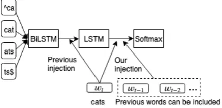
To deal with this problem, we propose an im-proved character-aware neural language model that takes into account the injected word-level information at the output layer. This model is strongly inspired by the success of n-gram lan-guage models. Our model can predict the next word using the embeddings of the words in the currentn-gram window, in addition to the hidden state of the LSTM layer. Specifically, we also use a gate to control how much word-level information should be taken before injecting it into the softmax function. After that, we combine the gated word-level information with the output of LSTM. Lastly, we feed these mixed information to the softmax function for word prediction. In our method, we can also take into account the information of previ-ous words when injecting word-level information into the softmax function.

im-plement1. We found our method effective com-pared with several common previous methods on 14 datasets with typologically diverse languages. In addition, the improvements can be further ob-tained when our injection method is used together with the previous methods. We also conducted a comprehensive comparison of these injection methods. Finally, we set up several experiments to check the effects of infrequent words on our model, and we also compared our model with sev-eral previous work on 6 common language model-ing datasets. Our results show that:

- Compared with the previous injection meth-ods (i.e., the gating mechanism, averaging, addition, and concatenation of word vectors), our injection method performs best on the majority of languages.

- Our injection method works effectively even when used alone, and the combination of our injection method and the previous injection methods performs better than the previous in-jection methods.

- When injecting word-level information into character-aware NLMs, discarding rare words in the training data can help improve the performance.

2 Related Work

Many work have attempted to improve character-aware NLMs in recent years. For example,

Assylbekov and Takhanov (2018) proposed sev-eral ways of reusing weights in character-aware NLMs. Gerz et al. (2018) achieved an improved result on 50 typologically diverse languages by in-jecting subword-level information into word vec-tors at the softmax. For a thorough review of past researches, readers are recommended to read the work byVania and Lopez(2017), who performed a systematic comparison across different models based on different subword units (characters, char-acter trigrams, BPE, etc.).

One direction related to our research is to in-ject word-level information into character-aware neural models. Aside from language modeling,

Santos and Zadrozny (2014) and dos Santos and Guimar˜aes(2015) first used a convolutional neural

1_{https://github.com/yukunfeng/char_}

word_lm

network (CNN) to encode characters and then con-catenated these encoded character-level represen-tations and word-level represenrepresen-tations for part-of-speech tagging and named entity recognition. Lu-ong and Manning(2016) introduced a character-word neural machine translation model that only consults character-level representations for rare words encoded with a deep LSTM.

As research efforts for language models, Kang et al. (2011) used a simple character-word NLM designed for Chinese. Miyamoto and Cho(2016) introduced a gate mechanism between word em-beddings and character emem-beddings obtained from a bidirectional LSTM (BiLSTM) for English. Ver-wimp et al.(2017) directly concatenated word and character embeddings without other subnetworks to encode the characters for English and Dutch.

Although there are a number of research efforts for using both character-level and word-level in-formation, they feed the two types of information only to LSTM, while our model also injects the word-level information into the softmax function. Previous work on this topic has usually been tested in a limited number of languages and lacks a com-prehensive comparison of different injection meth-ods. We will compare our method with the previ-ous methods mentioned in this section on 14 typo-logically diverse languages.

3 Model Description

For language modeling, we basically use a LSTM network (Hochreiter and Schmidhuber,1997). We denote the hidden state of LSTM for thet-th word wt as ht ∈ Rd, whered is the embedding size.

We incorporate word-level information using the neural network shown in Figure 1. We describe the details in the following subsections.

3.1 Input Word Representations

We use BiLSTM to encode charactern-grams to obtain character-level representation. We setnto 3 for all the languages except Japanese and Chi-nese, for which we set n to 1. This is because BiLSTM over character 3-grams obtained best re-sults on most LM datasets in the work ofVania and Lopez(2017), but Japanese and Chinese are more ideographic than the others, and it is expected that a smallernworks better.

Given a wordwt, we denote its embedding from

a lookup table Win ∈ Rd×|V| as wt ∈ Rd,

where|V|is the vocabulary size. We compute the character-level representation ofwtas follows:

ct=Wfhf w_l +Wbhbw0 +b, (1)

where hf w_l , hbw₀ ∈ Rd are the last states of the

forward and backward LSTMs respectively. Wf,

Wb ∈ Rd×d and b ∈ Rd are trainable

parame-ters. We define the following methods to obtain the combinationw0_tfromwtandct:

- gate: we use the same gating mechanism asMiyamoto and Cho (2016), which is de-scribed later to combinewtandct.

- avg, add, cat: we obtainw0_tthrough averag-ing, addition and concatenation ofwtandct,

respectively.

In the gating mechanism, we compute w0_t as fol-lows:

gin_wt = σ v>_gwt+bg

, (2)

w_t0 = (1−g_win_t)wt+gwintct, (3)

wherevg ∈Rdandbg ∈Rare trainable

parame-ters andσ(·)is a sigmoid function.

3.2 Representation of Input to Softmax

Our proposal is to combine ht with wt to better inform the softmax function of word-level infor-mation. Combinationh0_tis computed as follows:

h0_t=ht+gwoutt wt, (4)

where g_wout_t is a gate value. In our experiments, we set up two types of gate. One is a fixed value, gout_wt = 0.5. The other is similar to the definition in Eq. (2), which adaptively outputs a gate value depending onwt:

g_wout_t =σ

v>_kwt+bk

, (5)

wherev>_k ∈ _Rd_andb

k ∈ Rare trainable

param-eters. In Eq. (4), the gate is used only on word-level information to decide how much information wtshould be taken2.

In Eq. (4), if we remove the termht, the

resul-tant model is a simple word-level language model P(wt+1|wt). Based on this observation, we can

simply extend our method to contain the word-level information for previous words without extra parameters:

hword_t =

n X

i=1

1

iwt+1−i, (6)

where n is the number of the current and pre-vious words used to calculate hword_t . We sim-ply give smaller weights inversely proportional to distance i to the embeddings of the previous words. For example, whenn= 2,hword_t is com-puted aswt+ 1₂wt−1, which is used to calculate

P(wt+1|wt, wt−1). The hidden stateh0tnow can

be calculated as follows:

h0_t=ht+goutwt h word

t . (7)

3.3 Language Modeling

The language modeling task is to compute the probability of a given sentencew1, . . . , wT:

P(w1, . . . , wT) = T Y

t=1

P(wt|w1, . . . , wt−1).

(8) We use a softmax function based onh0_tto generate a probability distribution over the vocabulary:

P(wt+1|w1, . . . , wt) =softmax(WToutht0), (9)

where Wout ∈ Rd×|V| is output word

embed-dings.

4 Model Variants

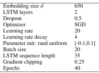
The hyper-parameters of our models are shown in Table1. The learning rate is decreased if no im-provement is observed in the validation dataset. Several baseline models and our models are listed as follows:

- Char-BiLSTM-LSTM: We use BiLSTM to encode characters without injecting word-level information.

2_{We have tested the above other methods, such as avg,}

add and cat, for combininghtandwt, in place of gate, and

Embedding sized 650

LSTM layers 2

Dropout 0.5

Optimizer SGD

Learning rate 20

Learning rate decay 4 Parameter init: rand uniform [-0.1,0.1]

Batch size 20

LSTM sequence length 35

Gradient clipping 0.25

Epochs 40

Table 1: Hyper-parameters of our model. We usedfor the sizes of the character/word embeddings and for the number of hidden units of LSTM and BiLSTM.

- Word-LSTM: Standard word-level LSTM model.

- Char-BiLSTM-gate/avg/add/cat-Word-LSTM: We combine character-level and word-level information at the input of LSTM through gate/avg/add/cat methods, mentioned in Sec.3.1.

- Char-BiLSTM-LSTM-Word: We inject word-level information only into the softmax function. This is our injection method.

- Char-BiLSTM-gate/avg/add/cat-Word-LSTM-Word: We combine our injection method and previous injection methods, which means we inject word-level informa-tion both at the input of LSTM and into the softmax function.

For both BiLSTM-LSTM-Word and Char-BiLSTM-gate/avg/add/cat-Word-LSTM-Word, we useg= 0.5/adaptive andn= 1/2/3to repre-sent our specific injection method. For example, Char-BiLSTM-LSTM-Word (g = 0.5, n = 2) represents that we use a fixed gate value on word-level information in Eq. (4) and we inject the information of the current word and the preceding word into the softmax function.

5 Experiments on 14 Languages

5.1 Datasets

Common language modeling datasets for evaluat-ing character-aware NLMs are from the work of

Botha and Blunsom(2014). While these datasets contain languages with rich morphology, they have only 5 different languages. Perhaps, the most large-scale language modeling datasets are from the work ofGerz et al.(2018), who released

50 language modeling datasets covering typolog-ically diverse languages. The difference between the newly released datasets and the previous com-mon datasets is that unseen words are kept in test set. Thus, on the datasets, we can test our methods in a real LM setup. The languages from the work ofGerz et al.(2018) were selected to represent a wide spectrum of different morphological systems and contain many low-frequency or unseen words. Thus, these datasets should be desirable for check-ing the performance of character-aware NLMs3.

To simplify the experiments without losing the wide coverage, we only chose datasets of 14 lan-guages from these datasets and tried to cover dif-ferent language typologies as well as difdif-ferent type/token ratios (TTRs). The statistics of our cho-sen datasets are shown in Table2. We used all the words observed in training data and one special unknown token for out-of-vocabulary words as the output vocabulary to make the setting the same as

Gerz et al.(2018).

5.2 Comparison of Baseline Models

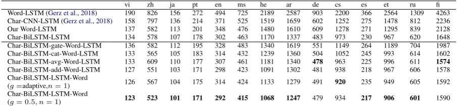
The results of Word-LSTM and Char-BiLSTM-LSTM are shown in Table 3. We also showed the results of Word-LSTM and Char-CNN-LSTM from the work of Gerz et al. (2018). The em-bedding size and the number of LSTM layers are the same as those for the models in Gerz et al. (2018). As shown in the table, both the Word-LSTM and Char-BiLSTM-LSTM baselines are better than the Word-LSTM and Char-CNN-LSTM from the work of Gerz et al. (2018) on all the datasets 4. Both Char-BiLSTM-LSTM and Char-CNN-LSTM from Gerz et al. (2018) are better than their respective Word-LSTM on all the datasets. One possible reason is that all the unseen words in the test set in the 14 datasets cannot be handled by Word-LSTM in the test-ing phase. However, character-aware models can encode the characters from these unseen words, making them possible to process these words. It is also shown that as TTR increases, Char-BiLSTM-LSTM achieves the better result than Word-LSTM. This may be because high-TTR lan-guages have more low-frequency words and un-seen tokens, as shown in Table2. Since frequent

3_{To test our models against previous work, we also}

in-clude experiments on common datasets, as described later.

4_{We have made the experimental setting the same as that}

Language Typology TTR Train vocab

#Train tokens

#Test tokens

#Unseen tokens

Freq<=15 (Train)

vi (Vietnamese) Isolating 0.04 32055 754K 61.9K 1678 8.50%

zh (Chinese) Isolating 0.06 43672 746K 56.8K 2132 16.00%

ja (Japanese) Agglutinative 0.06 44863 729K 54.6K 2558 15.20%

pt (Portuguese) Fusional 0.07 56167 780K 59.3K 2947 17.20%

en (English) Fusional 0.07 55521 783K 59.5K 3618 16.60%

ms (Malay) Isolating 0.07 49385 702K 54.1K 3918 16.00%

es (Spanish) Fusional 0.08 60196 781K 57.2K 3486 17.90%

he (Hebrew) Introflexive 0.12 83217 717K 54.6K 4855 27.20%

ar (Arabic) Introflexive 0.12 89089 722K 54.7K 6076 26.40%

de (German) Fusional 0.12 80741 682K 51.3K 5451 24.30%

cs (Czech) Fusional 0.14 86783 641K 49.6K 5436 30.00%

ru (Russian) Fusional 0.15 98097 666K 48.4K 4881 32.10%

et (Estonian) Agglutinative 0.17 94184 556K 38.6K 4960 33.70%

fi (Finnish) Agglutinative 0.20 115579 585K 44.8K 7899 38.10%

Table 2: The statistics of our language modeling datasets. TTR represents type/token ratio.

vi zh ja pt en ms he ar de cs es et ru fi

Word-LSTM (Gerz et al.,2018) 190 826 156 272 494 725 2189 2587 903 2200 366 2564 1309 4263 Char-CNN-LSTM (Gerz et al.,2018) 158 797 136 214 371 525 1519 1659 602 1252 275 1478 812 2236 Our Word-LSTM 137 582 113 201 348 476 1480 1610 609 1278 271 1295 839 2128 Char-BiLSTM-LSTM 134 578 107 178 302 463 1170 1337 483 973 230 967 620 1648 Char-BiLSTM-gate-Word-LSTM 136 582 112 195 328 483 1340 1619 551 1149 264 1189 704 1987 Char-BiLSTM-cat-Word-LSTM 133 565 105 183 314 432 1239 1360 504 1052 245 993 614 1602 Char-BiLSTM-avg-Word-LSTM 133 609 110 177 307 461 1181 1340 478 963 225 996 611 1574

Char-BiLSTM-add-Word-LSTM 127 551 103 171 298 423 1091 1302 481 938 218 967 606 1578 Char-BiLSTM-LSTM-Word

(g=adaptive,n= 1) 126 567 104 175 314 424 1133 1279 491 920 235 949 605 1592 Char-BiLSTM-LSTM-Word

(g= 0.5, n= 1) 123 523 101 171 292 415 1068 1247 479 934 217 906 601 1590

Table 3: Perplexity of several baseline models and Char-CNN-LSTM on 14 language modeling datasets. The best results among all models are in bold.

words still occupy the majority of both training and test data, injecting word-level information is still helpful for improving these character-aware models, as shown below.

5.3 Comparison of Different Injection Methods

The results of all the other different injection methods on 14 language modeling datasets are also shown in Table3. In our experiments, BiLSTM-gate-Word-LSTM underperforms Char-BiLSTM-LSTM on all the datasets. This in-dicates the gate method is not effective in our experiments. Char-BiLSTM-cat-Word-LSTM achieves better results than Char-BiLSTM-gate-Word-LSTM on all the datasets, but still under-performs Char-BiLSTM-LSTM on 8 out of 14 datasets. Char-BiLSTM-avg-Word-LSTM outper-forms Char-BiLSTM-cat-Word-LSTM on 9 out of 14 datasets, which indicates the simple aver-age method is better than the gating mechanism

and the concatenation method in our tasks. How-ever, Char-BiLSTM-avg-Word-LSTM still has no obvious improvements, compared with Char-BiLSTM-LSTM on most datasets.

We found some previous work also has similar results in the language modeling task. Kim et al.

(2016) used a Char-CNN-LSTM model without injecting word-level information. They reported that some basic methods (e.g., concatenation, av-eraging and adaptive weighting schemes) for in-jecting word-level information degraded the per-formance of their Char-CNN-LSTM. Miyamoto and Cho(2016) showed the concatenation method for injecting word-level information into their Char-BiLSTM-LSTM also degraded their Word-LSTM model.

than other previous injection methods in general in our tasks, while this simple method is less mentioned in the previous work. In conclusion, the performance of the previous injection methods in our experiments was in the descending order of add, avg, cat and gate.

Our Char-BiLSTM-LSTM-Word (g =

0.5, n = 1) and Char-BiLSTM-LSTM-Word (g = adaptive, n = 1) work effectively, and both of them achieve better results than Char-BiLSTM-LSTM. A simple fixed gate value in our injection method may be effective enough. Char-BiLSTM-LSTM-Word (g = 0.5, n = 1) works better than Char-BiLSTM-LSTM-Word (g = adaptive, n = 1) on most datasets. When compared with other injection methods, Char-BiLSTM-LSTM-Word (g = 0.5, n= 1) achieves the best results on most datasets (bold scores in Table3). This suggests that our injection method, aiming at the different position from the input of LSTM, the softmax function, makes good use of word-level information.

5.4 Combination of Injection Methods

To avoid too many combinations of our injec-tion method and other previous methods, we only chose to combine our Char-BiLSTM-LSTM-Word (g = 0.5, n = 1) with the other previous in-jection methods, because Char-BiLSTM-LSTM-Word (g= 0.5, n= 1) performs better than Char-BiLSTM-LSTM-Word (g = adaptive, n = 1), as mentioned above. The results of the combination of our Char-BiLSTM-LSTM-Word (g = 0.5, n= 1) and the previous injection methods are shown in Table4.

When our injection method is used together with gate/avg/cat/add methods, obvious im-provements can be observed on most datasets. Among them, Char-BiLSTM-add-Word-LSTM-Word (g = 0.5, n = 1) obtained the best results on most datasets (bold scores in Table4). The re-sult indicates that the previous injection methods do not make full use of word-level information, while our method, which injects the word-level in-formation into the different position, specifically, the softmax, can help the previous models make better use of the word-level information.

5.5 Including Word-level Information for Previous Words

As mentioned in Sec. 3.1, we can include word-level information for previous words when

inject-ing it into the softmax function. The number of words used in our injection method is denoted by n. In our experiments, we only setnto 1, 2 and 3, as we observed no obvious improvements when using a largern. Since Char-BiLSTM-add-Word-LSTM-Word (g = 0.5, n = 1) performs best in general on most datasets, as mentioned above, we only changednfor this model. Note that our Char-BiLSTM-add-Word-LSTM-Word (g = 0.5, n = 2/3) does not need extra parameters as we just reuse the word embeddings from the lookup ta-ble Win to compute word-level information. In

addition, the computational time of our injection method should be low, since the involved compu-tation is simple. The result is shown in Table5.

In general, Char-BiLSTM-add-Word-LSTM-Word (g = 0.5, n = 2) achieves the best re-sult on most datasets. Char-BiLSTM-add-Word-LSTM-Word (g = 0.5, n = 3) does not obtain further improvements on most datasets. Since our current method for including word-level informa-tion for previous words is simple, a more advanced method can be further exploited in future work.

5.6 Effects of Infrequent Words

In order to check whether infrequent words help our character-aware NLMs, we set up several ex-periments by discarding some infrequent words based on their word frequency. Note that we matain two independent vocabularies. One is the put vocabulary and is used to inject word-level in-formation. We obtain the word embeddings in our and previous injection methods through the lookup tableWin, as described in Sec.3.1. The other is

lan-vi zh ja pt en ms he ar de cs es et ru fi Char-BiLSTM-gate-Word-LSTM 136 582 112 195 328 483 1340 1619 551 1149 264 1189 704 1987 Char-BiLSTM-gate-Word-LSTM-Word

(g= 0.5, n= 1) 125 538 105 182 316 430 1339 1474 536 1116 260 1103 659 1728 Char-BiLSTM-cat-Word-LSTM 133 565 105 183 314 432 1239 1360 504 1052 245 993 614 1602 Char-BiLSTM-cat-Word-LSTM-Word

(g= 0.5, n= 1) 122 541 103 180 305 426 1158 1316 530 1031 241 1012 607 1561 Char-BiLSTM-avg-Word-LSTM 133 609 110 177 307 461 1181 1340 478 963 225 996 611 1574 Char-BiLSTM-avg-Word-LSTM-Word

(g= 0.5, n= 1) 121 495 99 165 293 398 1044 1224 488 890 218 898 569 1510 Char-BiLSTM-add-Word-LSTM 127 551 103 171 298 423 1091 1302 481 938 218 967 606 1578 Char-BiLSTM-add-Word-LSTM-Word

(g= 0.5, n= 1) 116 481 98 160 291 387 1038 1172 462 874 215 870 568 1494

Table 4: Perplexity of the combination of our injection method with the previous methods on 14 language modeling datasets.

vi zh ja pt en ms he ar de cs es et ru fi

Char-BiLSTM-add-Word-LSTM-Word

(g= 0.5, n= 1) 116 481 98 160 291 387 1038 1172 462 874 215 870 568 1494 Char-BiLSTM-add-Word-LSTM-Word

(g= 0.5, n= 2) 117 489 95 163 277 376 998 1179 452 867 213 884 548 1456 Char-BiLSTM-add-Word-LSTM-Word

(g= 0.5, n= 3) 118 475 96 162 285 391 1041 1162 463 877 215 913 563 1471

Table 5: Perplexity of our Char-BiLSTM-add-Word-LSTM-Word including word-level information for previous words on 14 language modeling datasets.

guage modeling task.

We denote the frequency threshold asθand set its value among 5, 15 and 25. If the frequency of a word seen in the training data is less than or equal to θ, we discard it. We refer the model that discards infrequent words as Char-BiLSTM-add-Word-LSTM-Word (g = 0.5, n = 1, θ = 5/15/25). The result is shown in Table7.

When discarding the words whose frequency is less than or equal to 15, the model obtains bet-ter results only on 2 out of 14 datasets than Char-BiLSTM-add-Word-LSTM-Word (g = 0.5, n = 1). This indicates some infrequent words are still helpful. When we increase the frequency thresh-old further to 25, the performance of the model has dropped compared with Char-BiLSTM-add-Word-LSTM-Word (g = 0.5, n = 1, θ = 15) as more frequent words are discarded. However, we found a relatively small frequency threshold θ = 5 works quite effectively. Char-BiLSTM-add-Word-LSTM-Word (g = 0.5, n = 1, θ = 5) achieves better results than Char-BiLSTM-add-Word-LSTM-Word (g = 0.5, n = 1) on 7 out of 14 datasets. It seems to be the trend that dis-carding infrequent words with θ = 5 is useful for high TTR languages. Note that we arranged our datasets from low TTR to high TTR in Table

7. Since many of the words in natural languages are rare as described in Zipf’s law, we can reduce the size of the input vocabulary significantly even with a smallθ. The size for the full input vocabu-lary and the reduced vocabuvocabu-lary with different

fre-quency threshold value is shown in Table 8. As we can see, whenθis set to 5, our model achieves better results with fewer parameters.

6 Experiments on 6 Common Datasets

In addition to the above datasets, we also set up 6 common language modeling datasets: English Penn Treebank (PTB) (Marcus et al.,1993) and 5 non-English datasets with rich morphology from the 2013 ACL Workshop on Machine Transla-tion5, which have been commonly used for eval-uating character-aware NLMs (Botha and Blun-som, 2014; Kim et al., 2016; Bojanowski et al.,

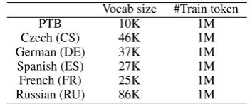
2017; Assylbekov and Takhanov, 2018). Since some of previous work has tested their model on PTB, we also included PTB in our experiment. We used the preprocessed small version of non-English datasets by Botha and Blunsom (2014) and followed the same split as the previous work. The data statistics is provided in Table9.

The results of our proposed models and previ-ous work are shown in Table 6. We used Char-BiLSTM-LSTM and Char-BiLSTM-add-Word-LSTM as baseline models. For our models, we set the frequency thresholdθto 5 and also setnto 2 as these settings help improve our character-aware NLMs, as discussed in Sec.5.6and Sec.5.5. The language models used in the previous work are im-proved at different aspects, and most of them are also based on standard LSTM, like ours. Botha

PTB CS DE ES FR RU

MLBL (Botha and Blunsom,2014) - 465 296 200 225 304

MorphSum (Kim et al.,2016) - 398 263 177 196 271

CharCNN (Kim et al.,2016) 78.9 371 239 165 184 261

SkipGram initialization (Bojanowski et al.,2017) - 312 206 145 159 206 MorphSum+RE+RW(Assylbekov and Takhanov,2018) 72.2 338 222 157 172 210

Char-BiLSTM-LSTM 85.5 311 198 144 164 223

Char-BiLSTM-add-Word-LSTM 79.1 300 199 138 155 213

Char-BiLSTM-add-Word-LSTM-Word

(g= 0.5, n= 1, θ= 5) 75.9 287 192 135 152 201

Char-BiLSTM-add-Word-LSTM-Word

(g= 0.5, n= 2, θ= 5) 76.1 284 193 137 150 202

Table 6: Perplexity of our models and previous work on 6 language modeling datasets.

vi zh ja pt en ms he ar de cs es et ru fi

Char-BiLSTM-add-Word-LSTM-Word

(g= 0.5, n= 1) 116 481 98 160 291 387 1038 1172 462 874 215 870 568 1494 Char-BiLSTM-add-Word-LSTM-Word

(g= 0.5, n= 1, θ= 5) 116 495 98 166 285 397 1016 1153 463 863 214 877 547 1492 Char-BiLSTM-add-Word-LSTM-Word

(g= 0.5, n= 1, θ= 15) 117 502 99 164 286 397 1046 1185 467 883 215 924 570 1492 Char-BiLSTM-add-Word-LSTM-Word

(g= 0.5, n= 1, θ= 25) 118 502 101 167 292 405 1053 1202 471 896 215 929 573 1526

Table 7: Perplexity of Char-BiLSTM-add-Word-LSTM-Word (g= 0.5, n= 1) with different frequency thresholds on 14 language modeling datasets.

Full θ= 5 θ= 15 θ= 25

vi 32055 5979 3383 2547

zh 43672 12200 5847 3940

ja 44863 9793 4355 2806

pt 56167 11207 4975 3203

en 55521 11142 5060 3282

ms 49385 9849 4728 3187

he 83217 14867 5961 3589

ar 89089 13459 5607 3482

de 80741 10290 4020 2511

cs 86783 12581 4680 2762

es 60196 11043 4722 2959

et 94184 10392 3815 2299

ru 98097 13337 4677 2734

fi 115579 11520 3930 2303

Table 8: The size of input vocabulary seen in the train-ing data on 14 datasets with different frequency thresh-old.

and Blunsom(2014) used the morphological log-bilinear (MLBL) model, which takes into account morpheme information. Kim et al. (2016) used CNN as their character encoder, and also trained an LSTM language model, where the input repre-sentation of a word is the sum of the morpheme embeddings of the word.Bojanowski et al.(2017) trained the word embeddings through skip-gram models with subword-level information, and used these word embeddings to initialize the lookup ta-ble of word embeddings of a word-level language

Vocab size #Train token

PTB 10K 1M

Czech (CS) 46K 1M

German (DE) 37K 1M

Spanish (ES) 27K 1M

French (FR) 25K 1M

Russian (RU) 86K 1M

Table 9: The data statistics of our 6 language modeling datasets.

model. Assylbekov and Takhanov(2018) focused on reusing embeddings and weights in a character-aware language model. The input of their model is also the sum of the morpheme embeddings of the word. As shown in the table, Char-BiLSTM-LSTM underperforms the previous work on PTB. One reason may be that we did not tune the parameters of our models on PTB. The hyper-parameters were simply kept the same in all the experiments on 20 datasets. As we can see, Char-BiLSTM-LSTM achieves better results than most previous work on non-English datasets. Our mod-els also achieve the best results on non-English datasets.

7 Conclusion

which is a widely used combination manner, we proposed to also inject word-level information into the softmax function in a character-aware neural language model. We gave a detailed compari-son with previous methods, and the result showed our proposal works effectively on typologically di-verse languages. For future work, it would be in-teresting to see how our model works for other tasks such as text generation.

Acknowledgments

We would like to thank anonymous reviewers for their constructive comments.

References

Zhenisbek Assylbekov and Rustem Takhanov. 2018. Reusing weights in subword-aware neural language models. InNAACL-HLT.

Yoshua Bengio, R´ejean Ducharme, Pascal Vincent, and Christian Jauvin. 2003. A neural probabilistic lan-guage model. Journal of machine learning research, 3(Feb):1137–1155.

Piotr Bojanowski, Edouard Grave, Armand Joulin, and Tomas Mikolov. 2017. Enriching word vectors with subword information. Transactions of the Associa-tion for ComputaAssocia-tional Linguistics, 5:135–146.

Jan Botha and Phil Blunsom. 2014. Compositional morphology for word representations and language modelling. InInternational Conference on Machine Learning, pages 1899–1907.

Katja Filippova, Enrique Alfonseca, Carlos A Col-menares, Lukasz Kaiser, and Oriol Vinyals. 2015. Sentence compression by deletion with lstms. In Proceedings of the 2015 Conference on Empirical Methods in Natural Language Processing, pages 360–368.

Daniela Gerz, Ivan Vuli´c, Edoardo Ponti, Jason Narad-owsky, Roi Reichart, and Anna Korhonen. 2018. Language modeling for morphologically rich lan-guages: Character-aware modeling for word-level prediction. Transactions of the Association of Com-putational Linguistics, 6:451–465.

Sepp Hochreiter and J¨urgen Schmidhuber. 1997. Long short-term memory. Neural computation, 9(8):1735–1780.

Moonyoung Kang, Tim Ng, and Long Nguyen. 2011. Mandarin word-character hybrid-input neural net-work language model. In Twelfth Annual Confer-ence of the International Speech Communication As-sociation.

Yoon Kim, Yacine Jernite, David Sontag, and Alexan-der M Rush. 2016. Character-aware neural language models. InAAAI, pages 2741–2749.

Philipp Koehn. 2009. Statistical machine translation. Cambridge University Press.

Wang Ling, Tiago Lu´ıs, Lu´ıs Marujo,

Ram´on Fern´andez Astudillo, Silvio Amir, Chris Dyer, Alan W. Black, and Isabel Trancoso. 2015. Finding function in form: Compositional character models for open vocabulary word representation. In EMNLP.

Minh-Thang Luong and Christopher D. Manning. 2016. Achieving open vocabulary neural machine translation with hybrid word-character models. In Proceedings of the 54th Annual Meeting of the As-sociation for Computational Linguistics (Volume 1: Long Papers), pages 1054–1063. Association for Computational Linguistics.

Mitchell Marcus, Beatrice Santorini, and Mary Ann Marcinkiewicz. 1993. Building a large annotated corpus of english: The penn treebank.

Tom´aˇs Mikolov, Martin Karafi´at, Luk´aˇs Burget, Jan ˇ

Cernock`y, and Sanjeev Khudanpur. 2010a. Re-current neural network based language model. In Eleventh annual conference of the international speech communication association.

Tomas Mikolov, Martin Karafi´at, Luk´as Burget, Jan Cernock´y, and Sanjeev Khudanpur. 2010b. Recur-rent neural network based language model. In IN-TERSPEECH.

Yasumasa Miyamoto and Kyunghyun Cho. 2016.

Gated word-character recurrent language model. In Proceedings of the 2016 Conference on Empirical Methods in Natural Language Processing, pages 1992–1997. Association for Computational Linguis-tics.

Cicero dos Santos and Victor Guimar˜aes. 2015. Boost-ing named entity recognition with neural character embeddings. InProceedings of the Fifth Named En-tity Workshop, pages 25–33. Association for Com-putational Linguistics.

Cicero D Santos and Bianca Zadrozny. 2014. Learning character-level representations for part-of-speech tagging. In Proceedings of the 31st International Conference on Machine Learning (ICML-14), pages 1818–1826.

Clara Vania and Adam Lopez. 2017. From characters to words to in between: Do we capture morphol-ogy? InProceedings of the 55th Annual Meeting of the Association for Computational Linguistics (Vol-ume 1: Long Papers), pages 2016–2027, Vancouver, Canada. Association for Computational Linguistics.