Index Terms—Smoothed particle hydrodynamics (SPH), Mitral valve, Lagrangian method, Fluid-structure interaction (FSI), Meshless method
Abstract— A numerical simulation for mechanical behavior of mitral valve was prepared by a particle approach: Smoothed Particle Hydrodynamics (SPH). The method was developed for this case as an important application of fluid-structure interaction problems. The simplicity and some further capabilities which have been shown in results highlighted the required assurance of using the SPH as reliable and simple tools for the wide range of hemodynamic problems.
I. INTRODUCTION
luid–structure interaction models are increasingly used in biomedical engineering applications and one of the most challenging fluid–structure problems that can be found in the human body involves the dynamics of heart valves. The most extensively studied valves are the mitral and the aortic valve. The former is a bileaflet valve located between the left atrium and left ventricle, the latter is a trileaflet and is located between the left ventricle and the aortic root. Both valves have extremely thin leaflets, which should hamper flow as little possible when opened, but need to prevent blood back-flow if closed. The arterial walls and heart muscle are compliant and therefore play an important role in the process of opening and closing. Altogether, the combination makes the problem extremely complex to model.
Different ways of modeling fluid–structure interaction (FSI) have been proposed in the past, each having its advantages and disadvantages. Arbitrary Lagrangian Eulerian (ALE) methods, as exploited by e.g. [1], are most commonly used for FSI problems and have the advantage to provide a strong coupling. As long as rotations, translations and deformations of the solid remain within certain limits,
Manuscript received March 5, 2011.
N. Amanifard is Associated Professor in Department of Mechanical Engineering, Faculty of Engineering, University of Guilan, Rasht, 3756 IRAN. (Corresponding author; phone: 6690274-8; fax: 98-131-6690271; e-mail: [email protected]).
B. Rahbar is with Department of Mechanical Engineering, Faculty of Engineering, University of Guilan, Rasht, 3756 IRAN (e-mail: [email protected]).
M. Hesan is with Department of Mechanical Engineering, Faculty of Engineering, University of Guilan, Rasht, 3756 IRAN (e-mail: [email protected]).
this method works very well and is recommended. However, for problems in which these limits are violated, elements become ill-shaped and ALE alone does not suffice. As a solution to this problem an often-used combination is ALE with some form of remeshing. This can, however, be a difficult and time consuming task. A more elegant way to solve the system allowing free movements of a structure through a fluid domain was proposed by Peskin [2]. He introduced a method that later became known as the immersed boundary method (IBM) [3] where flow-induced solid body motions could be computed without adjusting the fluid grid/mesh. By defining a set of interconnected points related to each other by some elastic law local body forces were enforced to the fluid. Extensions of this model to three dimensional heart (valve) problems were published in e.g. [4] and the method is still used in many fields.
A method that resembles the above mentioned methods was introduced [5] for slender deforming bodies. In this method a fluid mesh is considered with an immersed solid mesh, and the solid mesh and fluid mesh are coupled by a Lagrange multiplier (or local body forces) at the boundary of the solid. The elegance of this method is its simplicity and flexibility. Stijnen et al. [6] introduced a model for mechanical heart valves using this fictitious domain method. The model was capable of computing a full cardiac cycle, using the fact that the position of a closed mechanical heart valve is known a priori. By creating the fluid mesh such that a curve of fluid edges coincided with the solid boundary in the closed state, the occurring drop in pressure across the valve could be described. Recently, fictitious domain methods have been proposed that are not restricted to slender bodies by introducing Lagrange multipliers across the whole solid body instead of only along its boundaries [7]. This enables the computation of a pressure drop across the solid body without alignment of the meshes and such makes the method suitable for a wider range of applications.
Using lagrangian description for both fluid and solid domain is another remedy to the simulation of FSI problems, and Smoothed Particle Hydrodynamics (SPH) is one of the methods. In approaches mentioned above, mesh generation for the problem domain is a prerequisite for the numerical simulations. Therefore, the idea of eliminating the mesh has evolved naturally. SPH is a fully lagrangian mesh-less method that originally developed for astrophysical problems by Lucy [8], and separately by Gingold and Monaghan [9] and later extended to model a
Numerical Simulation of the Mitral Valve
Opening Using Smoothed Particle
Hydrodynamics
Nima Amanifard, Behnam Rahbar, Muhammad Hesan
wide range of problems. In this approach a continuum domain is replaced with a set of particles which can carry the mass, density, velocity, and other material information. The interactions between these particles are determined by interpolation from information at SPH particles. Confronting with complex physics such as FSI, SPH shows great ability from itself [10].
In current study, fully explicit two steps SPH method is used to simulate two dimensional model of heart mitral valve with the pulsatile flow.
II. GOVERNING EQUATIONS
Simulation of considered problem consists of two domains, fluid and solid. Both fluid and solid media are assumed to be isothermal and incompressible.
Governing equations for fluid domain in absence of body forces may be written as:
j j
x
u
Dt
D
∂
∂
−
=
ρ
ρ
(1)
j j
ij i
x
P
x
Dt
Du
∂
∂
−
∂
∂
=
ρ
τ
ρ
1
1
(2)where j j
u
P
t
x
,
,
ρ
,
,
andτ
ij denotes thej
th componentof position vector, time, density, pressure, velocity vector, and shear stress tensor, respectively.
For solid domain, beside the continuity equation, the momentum equation for an elastic body is as follows:
j ij i
x
Dt
Du
∂
∂
=
σ
ρ
1
(3)where
σ
ij is the stress tensor. The stress tensor can bedecomposed into its isotropic and deviatoric parts:
ij ij ij
S
P
+
−
=
δ
σ
(4)where kk
/
3
P
=
−
σ
is pressure,S
ij is the deviatoric stresstensor and
δ
ij is the Kronecker tensor.The linear elastic relation between stress and deformation tensors can be derived in time in order to obtain an evolution equation for ij
S
. The use of the corotational, orJaumann, time derivative guarantees that the formulation is independent from superposed rigid rotations, resulting in the incremental formulation of Hook’s law corrected by the Jaumann rate [10]:
kj ik jk ik ij ij ij ij
S
S
G
Dt
DS
ε
δ
ε
+
ω
+
ω
−
=
3
1
2
(5)where
∂
∂
+
∂
∂
=
ji ij ijx
u
x
u
2
1
ε
(6)is the rate of deformation tensor,
∂
∂
−
∂
∂
=
ji ij ijx
u
x
u
2
1
ω
(7)is the spin tensor and G is the shear modulus.
III. FUNDAMENTALS
A. Interpolation
The main features of the SPH method, which is based on integral interpolants [11]. In SPH, the fundamental principle is to approximate any function F(r) by
(
r
r
h
)
d
r
W
r
F
r
F
(
)
=
∫
(
′
)
−
′
,
′
(8)where h is called the smoothing length and
W
(
r
−
r
′
,
h
)
isthe weighting function or kernel. This approximation, in discrete notation, leads to the following approximation of the function at a particle (interpolation point) a,
∑
=
bab b b
b
W
F
m
r
F
ρ
)
(
(9)where the summation is over all the particles within the region of compact support of the kernel function. The mass and density are denoted by
m
b andr
b respectively and)
,
(
r
r
h
W
W
ab=
a−
b is the weight function or kernel.B. Kernel
The performance of an SPH model is critically dependent on the choice of the weighting functions. They should satisfy several conditions such as positivity, compact support, and normalization. Also,
W
ab must bemonotonically decreasing with increasing distance from particle a and behave like a delta function as the smoothing length, h, tends to zero [11]. Kernels depend on the smoothing length, h, and the non-dimensional distance between particles given by
h
r
q
=
, r being the distancebetween particles a and b. The parameter h, often called influence domain or smoothing domain, controls the size of the area around particle a where contribution from the rest of the particles cannot be neglected.
In the literature many possible forms for smoothing function have been proposed ranging from Gaussian functions to spline functions with the compact condition. In this study the cubic spline kernel in two dimensions is used:
≥
≤
≤
−
≤
−
+
=
2
0
2
1
)
2
(
28
10
1
4
3
2
3
1
7
10
3 2
3 2 2
q
q
q
h
q
q
q
h
W
abπ
π
(10)
C. Gradient and Divergence
The gradient and divergence operators need to be formulated in accordance with the SPH concept. In the current work, the following commonly used forms are employed for the gradient of a scalar F and the divergence of a vector u[12]:
ab a
b b
b
a a b a
a
W
F
F
m
F
∇
+
=
∇
∑
2 21
ρ
ρ
ab a b b i b a i a b i a a a
W
u
u
m
u
⋅
∇
+
=
⋅
∇
∑
2 21
ρ
ρ
ρ
(12)where
∇
aW
ab is gradient of the kernel function)
,
(
r
r
h
W
a−
b with respect tor
a, the position of particle a.D. Laplacian formulation
A simple way to formulate the Laplacian operator is to envisage it as dot product of the divergence and gradient operators. This approach proved to be problematic since second derivative of the kernel is very sensitive to particle disorder and can easily lead to pressure instability and decoupling in the computation due to the co-location of the velocity and pressure. In this paper, the following alternative approach is adopted [13]:
(
)
2 2 28
1
η
ρ
ρ
ρ
+
∇
⋅
+
=
∇
⋅
∇
∑
ab ab a ab ab b a b b br
W
r
F
m
F
(13)IV. SOLUTION ALGORITHM
Solution of governing equations of two media of fluid and solid in order to acquisition of velocity and pressure fields decompose into two steps as in specified by Hosseini et al. [14]. First step has the role of predictor and the stress tensor is calculated in this step.
Fluid domain: In this step, the divergence of the shear stress tensor i
f
T
is calculated [15]:)
.(
)
(
)
(
)
(
4
1
2 2 2 b ab a b ab
ab a ab b a b
u
u
r
W
r
m
j
x
ij
i
f
T
−
+
+
∇
⋅
+
=
∂
∂
=
∑
η
ρ
ρ
µ
µ
τ
ρ
(14)where
)
(
1
)
,
(
a bab ab b a a ab
a
r
r
r
dr
dW
h
r
r
W
W
=
∇
−
=
−
∇
(15)Solid domain: In the first step for solid domain, the divergence of deviatoric stress tensor i
s
T
is calculated in accordance with equation (5),∑
+
⋅
∇
=
∂
∂
=
a abb ij b a ij a b j ij i s
W
S
S
m
x
S
T
1
(
2 2)
ρ
ρ
ρ
(16)At the end of the first step, for each domain, intermediate velocity and position vectors are obtained separately:
t
T
u
u
∗=
t+
⋅
∆
(17)t
u
r
r
*=
t+
*⋅
∆
(18)Thus far no constraint has been imposed to satisfy the incompressibility of the fluid and it is expected that the density of some particles change during this updating. In fact, with the help of the continuity equation one can calculate the density variations of each particle as
∑
−
⋅
∇
=
b ab a i b a b b a aW
u
u
m
Dt
D
)
(
* *
ρ
ρ
ρ
(19)The velocity field i
u
ˆ
which is needed to restore thedensity of particles to their original value is now calculated. To do this, in the second step of the algorithm, the momentum equation with the pressure gradient term as a source term is combined with the continuity equation (1) as
0
ˆ
.
1
* 0 0=
∇
+
∆
−
iu
t
ρ
ρ
ρ
(20)t
P
u
ˆ
i=
−
(
1
*∇
)
∆
ρ
(21)To obtain the following pressure Poisson equation
2 0 * 0 *
)
1
.(
t
P
∆
−
=
∇
∇
ρ
ρ
ρ
ρ
(22)Equation (22) can be discretized according to equation (13) to obtain the pressure of each particle as
)
)
(
8
/(
)
)
(
8
(
2 2 2 2 2 2 2 0 * 0∑
∑
+
∇
⋅
+
+
∇
⋅
+
+
∆
−
=
b ij ab a ab b a b b ij ab a ab a b a b ar
W
r
m
r
W
r
P
m
t
P
η
ρ
ρ
η
ρ
ρ
ρ
ρ
ρ
(23)Using equation (23) for the pressure of each particle one can calculate according to equations (20) and (11) as
∑
+
∇
∆
−
=
b ab a b b a a b aW
P
P
m
t
u
ˆ
(
2)
*2
ρ
ρ
(24)Finally, the velocity of each particle at the end of time-step will be obtained as
u
u
u
t tˆ
*
+
=
∆ +
(25) The particles are moved using XSPH variant that moves a particle with a smooth velocity that is closer to average velocity among its neighborhoods [16]:ab t t a b
b a b
b t t a t t
a
u
u
W
m
u
u
(
)
)
(
2
ˆ
+∆ +∇−
+∆+
+
=
∑
ρ
ρ
ε
(26)where
ε
is a constant in the range of(
0
<
ε
<
1
)
. The final positions of particles are calculated using a central difference scheme in time:)
ˆ
(
2
t a t t a t t ta
u
u
t
r
r
+∆=
+
∆
+∆+
(27)V. BOUNDARY CONDITION
In this paper, two types of boundary conditions were defined, velocity inlet and no-slip boundary condition. At the inlet, a pulsatile flow with the form of
)
sin(
max
t
u
u
=
ω
has been considered in whichu
max isthe maximum velocity,
ω
is the frequency andt
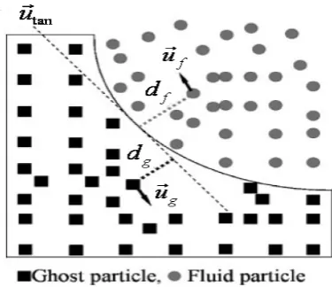
is the time.Fig. 1. Construction of artificial velocity for boundary particles to simulate a no-slip boundary condition.
In order to implement the aforementioned method for FSI problems, it can be assumed that there are ghost particles which have similar positions as wall particles. The artificial extrapolated velocity of each wall particle is attributed to the relevant ghost particle. Other properties of these ghost particles are similar to those of fluid particles.
)
)(
(
tantan if
i
g f i i
g
u
u
d
d
u
u
=
+
−
(28)The no-slip boundary condition satisfies when velocity of ghost particles as well as boundary particles are contributed to calculate viscous forces [18].
VI. TEST CASE
The numerical test case is a two dimensional FSI simulation of the mitral valve opening in a fluid canal. A two dimensional model of leaflet is shown in Fig. 2 and essential boundary conditions are as follows:
,
0
4
,...,
1
0
,
)
2
sin(
1
.
0
,
0
1 2
3 1
1 1
s s
f i f
f f
f f
at
u
i
with
at
u
at
T
t
u
at
u
Ω
∂
=
=
Ω
∂
=
Ω
∂
=
Ω
∂
=
π
[image:4.595.60.248.63.225.2](29)
Fig. 3. Schematic representation of the solid and fluid including the relevant geometric parameters.
TABLEI
GEOMETRIC AND MATERIAL PARAMETERS FOR THE NUMERICAL SIMULATION
Wf (cm) 15.0
Hf (cm) 2.0
Hs (cm) 1.9
W1s (cm) 1.0
W2s (cm) 5×10⁻²
μ (Pa.s) 4×10⁻³
ρ (kg/m3) 1056
T (s) 1.0
G (Pa) 1.2×10⁶
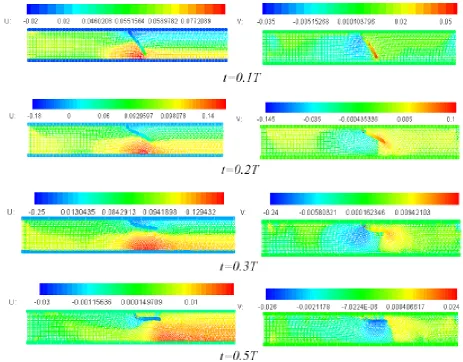
with f
(
1f,
2f)
u
u
u
=
. In Fig. 3 the relevant dimensionalparameters are given and the values of geometric and material parameters are shown in table I. The leaflet positions and the staggered plot of velocity field are shown in fig. 4 and fig. 5 respectively at different stages of the flow pulse.
[image:4.595.309.548.197.350.2] [image:4.595.48.266.490.682.2]REFERENCES
[1] C.W. Hirt, A.A. Amsden, J.L. Cook, “An arbitrary Lagrangian– Eulerian computing method for all speeds,” J. Comput. Phys, vol. 14,
pp. 227–253, 1974
[2] C.S. Peskin, “Flow patterns around heart valves: a numerical method,”
J. Comput. Phys, vol. 10, pp. 252–271, 1972
[3] C.S. Peskin, “The immersed boundary method,” Act. Num. vol. 11, pp.
479–517, 2002.
[4] D.M. McQueen, C.S. Peskin, “Shared-memory parallel vector implementation of the immersed boundary method for the computation of blood flow in the beating mamalian heart,” J. Supercomput, vol. 11,
pp. 213–236, 1997.
[5] J. de Hart, G.W.M. Peters, P.J.G. Schreurs, F.P.T. Baaijens, “A two-dimensional fluid–structure interaction model of the aortic value,” J.
Biomech, vol. 33, pp. 1079–1088, 2000.
[6] J.M.A. Stijnen, J. de Hart, P.H.M. Bovendeerd, F.N. van de Vosse, “Evaluation of a fictitious domain method for predicting dynamic response of mechanical heart valves,” J. Fluid Struct, vol. 19, pp. 835–
850, 2004.
[7] X. Shi, N. Phan-Thien, “Distributed Lagrange multiplier/fictitious domain method in the framework of lattice Boltzmann method for fluid– structure interactions,” J. Comput, vol. 206, pp. 81–94, 2005.
[8] L.B. Lucy, “A numerical approach to the testing of the fission hypothesis,” J. Astron., vol. 82, pp. 1013–1024, 1977.
[9] R.A Gingold, J.J. Monaghan, “Smoothed particle hydrodynamics: theory and application to non-spherical stars,” Mon. Not. R. Astron.
Soc., vol. 181, pp. 375–389, 1977.
[10] C. Antoci, M. Gallati, S. Sibilla, “Numerical simulation of fluid– structure interaction by SPH,” Computers and Structures, vol. 85, pp.
879–890, 2007.
[11] J. J. Monaghan, “Smoothed particle hydrodynamics,” Ann. Rev. Astron.
Astrophys, vol. 30, pp. 543–574, 1992.
[12] A. Colagrossi, M. Landrini, “Numerical simulation of interfacial flows by smoothed particle hydrodynamics,” J. Comput. Phys., vol. 191, pp.
448–475, 2003.
[13] S.J. Cummins, M. Rudman, “An SPH projection method” J. Comput.
Phys., vol. 152, pp. 584–607, 1999.
[14] S.M. Hosseini, M.T. Manzari, S.K. Hannani, “A fully explicit three step SPH algorithm for simulation of non-Newtonian fluid flow,” Int. J. of
Numerical Methods for Heat and Fluid Flow, vol. 17, pp. 715–735,
2007.
[15] Shao S.D, Lo E.Y.M., “Incompressible SPH method for simulating Newtonian and non-Newtonian flows with a free surface,” Advances in
Water Resources, vol. 26, pp. 787–800, 2003.
[16] J.J. Monaghan, “On the problem of penetration in particle methods,” J.
Comput. Phys., vol. 82, pp. 1–15, 1989.
[17] J. P. Morris, P. J. Fox, Y. Zhu, “Modeling low Reynolds number incompressible flows using SPH,” J. Comp. Phys., Vol. 136, pp. 214–
226, 1997.
[18] M. H. Farahani, N. Amanifard, Gh. Pouryoussefi, “Numerical Simulation of a Pulsatory Flow Moving Through Flexible Walls Using Smoothed Particle Hydrodynamics,” Proceedings of the World
[image:5.595.60.524.59.421.2]Congress on Engineering 2008, pp. 1–5.