Reliability Measurement without Limits
Dennis Reidsma
∗University of Twente
Jean Carletta
∗∗ University of EdinburghIn computational linguistics, a reliability measurement of 0.8 on some statistic such as κ is widely thought to guarantee that hand-coded data is fit for purpose, with 0.67 to 0.8 tolerable, and lower values suspect. We demonstrate that the main use of such data, machine learning, can tolerate data with low reliability as long as any disagreement among human coders looks like random noise. When the disagreement introduces patterns, however, the machine learner can pick these up just like it picks up the real patterns in the data, making the performance figures lookbetter than they really are. For the range of reliability measures that the field currently accepts, disagreement can appreciably inflate performance figures, and even a measure of 0.8 does not guarantee that what looks like good performance really is. Although this is a commonsense result, it has implications for how we work. At the very least, computational linguists should lookfor any patterns in the disagreement among coders and assess what impact they will have.
1. Introduction
In computational linguistics, 0.8 is often regarded as some kind of magical reliability cut-off guaranteeing the quality of hand-coded data (e.g., Reithinger and Kipp 1998; Shriberg et al.1998; Galley et al.2004), with 0.67 to 0.8 tolerable—although it is as often honored in the breech as in the observance.The argument for the meaning of 0.8 arises originally from Krippendorff (1980, page 147), in a comment about practice in the field of content analysis.He states that correlations found between two variables using their hand-coded values “tend to be insignificant” when the hand-codings have a reliability below 0.8. He uses a specific reliability statistic, α, for his measurements, but Carletta (1996) implicitly assumes kappa-like metrics are similar enough in practice for the rule of thumb to apply to them as well.A detailed discussion on the differences and similarities of these, and other, measures is provided by Krippendorff (2004); in this article we will use Cohen’sκ(1960) to investigate the value of the 0.8 reliability cut-off for computational linguistics.
Modern computational linguists use data in a completely different way from 1970s content analysts.Rather than correlating two variables, we use hand-coded data as
∗University of Twente, Human Media Interaction, Room ZI2067, PO Box 217, NL-7500 AE Enschede, The Netherlands, [email protected].
∗∗University of Edinburgh, Human Communication Research Centre, [email protected].
training and test material for automatic classifiers.The 0.8 rule of thumb is irrelevant for this purpose, because classifiers will be affected by disagreement differently than correlations.Furthermore, Krippendorff’s argument comes with a caveat: the disagree-ment must be due to random noise.For his case of correlations, any patterns in the disagreement could accidentally bolster the relationship perceived in the data, leading to false results.To be sure that data is fit for the intended purpose, Krippendorff advises the analyst to look for structure in the disagreement and consider how it might affect data use.Although computational linguists have rarely followed this advice, it is just as relevant to us.Machine-learning algorithms are designed specifically to look for, and predict, patterns in noisy data.In theory, this makes random disagreement unimportant. More data will yield more signal and the learner will ignore the noise.However, as Craggs and McGee Wood (2005) suggest, this also makes systematic disagreement dangerous, because it provides an unwanted pattern for the learner to detect.We demonstrate that machine learning can tolerate data with a low reliability measurement as long as the disagreement looks like random noise, and that when it does not, data can have a reliability measure commonly held to be acceptable but produce misleading results.
2. Method
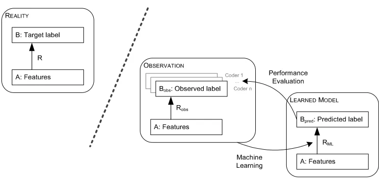
[image:2.486.48.434.441.625.2]To explain what is wrong with using 0.8 as a cut-off, we need to think about how data is used for classification tasks.Consider Figure 1, which shows a relation between some featuresAand a class labelB.Learning labels from a set of features is a common task in computational linguistics; for instance, in Shriberg et al.(1998), which assumes a pre-existing dialogue act segmentation, the labels are dialogue act types, and they are learned from automatically derived prosodic features.In this way of using data, only one of the variables—the output dialogue act label—is hand-coded.In the figure, the real relationship between prosody and dialogue act label is shown on the left;Rrelates the prosodic featuresAto the output actB.
Figure 1
In theory, there is one correct label for any given act.However, in practice hu-man coders disagree, choosing different labels for the same act (sometimes even with divergences that make one question whether there is one correct answer).The data actually available for analysis is shown in the middle of the figure.Here, the automatic features, A, are the same as before, but there are multiple, possibly differing labels for the same act, Bobs, coming from different human annotators.Finally, on the right the figure shows the classifier.It takes the same prosodic features Aand uses them to predict a dialogue act labelBpredon new data, using the relationship learned from the
observed data, RML.Projects vary in how they choose data from which to build the
classifier when coders disagree, but whatever they do is colored by the observations they have available to them.We often think of reliability assessment as telling us how much disagreement there is among the human coders, but the real issue is how their individual interpretations of the coding scheme makeRMLdiffer fromR.
There is a problem that arises for anyone using this methodology.Without the “real” data, it is impossible to judge how well the learned relationship reflects the real one.Classification performance forBpredcan only be calculated with respect to the
“ob-served” dataBobs.In this article, we surmount this problem by simulating the real world
so that we can measure the differences between this “observed” performance and the “real” performance.Our simulation uses a Bayesian network (Pearl 1988) to create an initial, “real” data set with 3,000 samples of features (A) and their corresponding target labels (B).For simplicity, we use a single five-valued feature and five possible labels. The relative label frequencies vary between 17% and 25%.This gives us a small amount of variation around what is essentially equally distributed data.We corrupt the labels (B) to simulate the “hand-coded” observed data (Bobs) corresponding to the output of
a human coder, and then train a neural network constructed using the WEKA toolkit (Witten and Frank 2005) on 2,000 samples from Bobs.Finally, we calculate the neural
network’s performance twice, using as test data either the remaining 1,000 samples from Bobsor the initial, “real” versions of those same 1,000 samples.
There are three ways in which we need to vary our simulation in order to be sys-tematic.The first is in the strength of the relationship between the features the machine learner takes as input and the target labels, which we achieve simply by changing the probabilities in the Bayesian network that creates the data set.In the simulation, we vary the strength of the relationship in eight graded steps.1The second is in theamount of disagreement we introduce when we create the observed data (Bobs).We create 200 different versions of the hand-coded data that cover a range of values from κ=0 to
1 We use Cramer’s phi to measure the strength of a relationship.Cramer’s phi is defined as
φc=
χ2 (N)∗dfsmaller
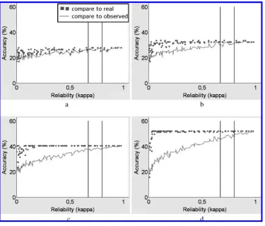
Figure 2
Machine-learning performance obtained on annotations with noise-like disagreements for (a) weak (φc=0.06), (b) moderate (φc=0.20), (c) strong (φc=0.32), and (d) very strong (φc=0.45) relationships between the features and labels.
κ=1, by introducing a varying amount of observation errors in the simulated coding process.2The third is in thetypeof disagreement with which we degrade the real data to create the observed data (Bobs), representing the types of coding errors the human
annotators make.Again for simplicity, we describe the effects of both random errors and the overuse of a single coding label.
3. The Case ofNoise
Figure 2 shows how a neural network performs when coders make random mistakes in their coding task, that is, for noise-like disagreement, for the cases of (a) weak, (b) moderate, (c) strong, and (d) very strong relationships between the features (A) and labels (B).Here, theyaxis shows “accuracy,” or the percentage of samples in the test
data for which the network chooses the correct label.The xaxis varies the amount of coder errors in the data to correspond to different κ values, with the two black lines marking the values ofκ=0.67 andκ=0.8.
Look first at the series depicted as a line.It shows accuracy measured by using the “observed” version of the test data, which is how testing is normally done.For each relationship strength, asκincreases, so does accuracy.In all cases, atκ=0 (that is, when the coders fail to agree beyond what one would expect if they were all choosing their labels randomly) accuracy is at 20%, which is what one would expect if the classifier were choosing randomly as well.For any given κ value, the stronger the underlying relationship, the more benefit the neural network can derive from the data.Now look at the other of the two series, depicted as small squares.It shows accuracy measured by using the “real” version of the data.Interestingly, the “real” performance, that is, the power of the learned model to predict reality, is higher than performance as measured against the observed data.This is because for some samples, the classifier’s predictions are correct, but because the observations contain errors, the test data actually gets them wrong.The stronger the relationship in the real data, the more marked this effect becomes.The neural network is able to disregard noise-like coding errors at very low κvalues simply because the errors contain no patterns for it to learn.
4. The Case ofOverusing a Label
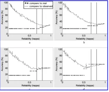
Now consider the case where instead of random coding errors, the coder over-uses the least frequent one of the five labels forB.Figure 3 shows the results for this kind of coding error.Remember that in the graphs, the series depicted as a line shows the observedperformance of the classifier—that is, performance as it is usually measured. The two black lines again mark theκvalues of interest (κ=0.67 andκ=0.8).
The graphs show an entirely different effect from the one obtained for noise-like coding errors: For lower values ofκ, the observed performance is spuriously high.This makes perfect sense—κis low when the pattern of label overuse is strong, and the neural network picks it up.When the observed data is used to test performance, some of the samples match not because the classifier gets the label right, but because it overuses the same label as the human coder.For data with a very strong correlation between the input featuresAand the output labelsB, the turning point below which performance is spuriously high occurs at aroundκ=0.55 (Figure 3d), a value the community holds to be pretty low but which is not unknown in published work.However, when the underlying relationship to be learned is moderate or strong (Figures 3b and 3c), the spuriously high results already occur forκvalues commonly held to be tolerable.With a weak relationship, the turning point can occur atκ >0.8 (Figure 3a).
5. Discussion
Figure 3
Machine-learning performance obtained on annotations that suffered from over-coding for (a) weak (φc=0.06), (b) moderate (φc=0.20), (c) strong (φc=0.32), and (d) very strong (φc=0.45) relationships between the features and labels.
learn vary in strength.This makes discerning the degree of danger more difficult, but does not change the substance of our argument.
Although the graphs we show are for a specific simulation, the general pattern we describe is robust.In particular, usingα in place ofκdoes not markedly change the results; neither does increasing or decreasing the data set size.Our simulations and results are presented for a machine-learning context.However, that does not mean that other types of data use are immune to the problems we describe here.Other statistical uses of data will be affected in their own ways by the difference between structural and noise-like disagreement.
6. Implications
and Romera 1999; Di Eugenio and Glass 2004; Artstein and Poesio 2005).Computational linguists are of course aware that no overall reliability measure can give a complete story, but often fail to spend time analyzing coder disagreements further.Unfortunately, our results suggest that current practice is insufficient, at least where the data is destined to be input for a machine-learning process and quite possibly for other data uses as well.This complements observations of Artstein and Poesio: Besides the fact that many different ways of calculating reliability metrics lead to different values, which makes comparing them to a threshold difficult (Artstein and Poesio in press), the very idea of having any such single threshold in the first place turns out to be impossible to hold.Instead of worrying about exactly how much disagreement there is in a data set and how to measure it, we should be looking at the form the disagreement takes. A headline measurement, no matter how it is expressed, will not show the difference between noise-like and systematic disagreement, but this difference can be critical for establishing whether or not a data set is fit for the purpose for which it is intended.
To tease out what sort of disagreement a data set contains, Krippendorff suggests calculating odd-man-out and per-class reliability to find out which class distinctions are problematic (1980, page 150).Bayerl and Paul (2007) discuss methods for determining which factors (schema changes, coding team changes, etc.) were involved in causing poor annotation quality.Wiebe, Bruce, and O’Hara (1999) suggest looking at the mar-ginals and how they differ between coders to find indications of whether disagreements are caused by systematic bias (as opposed to being random) and in which classes they occur.Although clearly useful techniques, none of these diagnostics is specifically designed to address the needs of machine learners which are designed to recognize pat-terns.Overusing a label is just one simple example of a type of systematic disagreement that adds unwanted patterns that a machine learner can find.Any spurious pattern could be a problem.For this reason, we should be looking specifically for patterns in the disagreement itself.
Our suggestion for one possible diagnostic technique is based on the following observation: If the disagreements between two coders containnopattern, any test for association or correlation, when performed on only the disagreed items, should show no relation between the labels assigned by the two coders.For certain patternsin the disagreement, however, a correlation would show up.(To see this, consider the case where one coder tends to label rhetorical questions as yes/no-questions and the other coder assigns both labels correctly: If this happens often enough, tests for association would come up with a relation between the labels for the two coders for the disagreed items.) If the test shows a correlation, the disagreements add patterns for the machine learner to find.Unfortunately, the converse does not necessarily hold: It is possible that not all patterns that could be picked up by a machine learner will show up in correlations between disagreed items, for example because the amount of multiply-annotated data is too small.The computational linguistics community therefore needs to develop additional diagnostics for patterns in the coder disagreements.
reliability for that particular label will be the most important.Finally, different machine-learning algorithms may react differently to different kinds of patterns in the data and to combinations of patterns in different relative strengths.In complicated cases, perhaps the safest way to assess whether or not there is a problem with systematic disagreement is to run a simulation like the one we have reported but with the kind and scale of disagreement suspected of the data, and to use that to estimate the possible effects of unreliable data on the performance of machine-learning algorithms.
Acknowledgments
We thank Rieks op den Akker, Ron Artstein, and Bonnie Webber for discussions that have helped us frame this article, as well as the anonymous reviewers for their thoughtful comments.This work is supported by the European IST Programme Project FP6-033812 (AMIDA, publication 36).This article only reflects the authors’ views and funding agencies are not liable for any use that may be made of the information contained herein.
References
Aron, Arthur and Elaine N.Aron.2003. Statistics for Psychology.Prentice Hall, Upper Saddle River, NJ.
Artstein, Ron and Massimo Poesio.2005. Bias decreases in proportion to the number of annotators.InProceedings of FG-MoL 2005, pages 141–150, Edinburgh.
Artstein, Ron and Massimo Poesio.In press. Inter-coder agreement for computational linguistics.Computational Linguistics. Bayerl, Petra Saskia and Karsten Ingmar
Paul.2007.Identifying sources of disagreement: Generalizability theory in manual annotation studies. Computational Linguistics, 33(1):3–8. Carletta, Jean C.1996.Assessing agreement
on classification tasks: The kappa statistic. Computational Linguistics, 22(2):249–254. Cohen, Jacob.1960.A coefficient of
agreement for nominal scales.Educational and Psychological Measurement, 20(1):37–46. Cohen, Jacob.1988.Statistical power analysis
for the behavioral sciences, 2nd edition. Lawrence Erlbaum, Hillsdale, NJ. Craggs, Richard and Mary McGee Wood.
2005.Evaluating discourse and dialogue coding schemes.Computational Linguistics, 31(3):289–296.
Di Eugenio, Barbara and Michael Glass. 2004.The kappa statistic: A second look. Computational Linguistics, 30(1):95–101. Galley, Michel, Kathleen McKeown, Julia
Hirschberg, and Elizabeth Shriberg. 2004.Identifying agreement and disagreement in conversational speech:
Use of Bayesian networks to model pragmatic dependencies.InProceedings of the 42nd Meeting of the Association for Computational Linguistics (ACL–04), pages 669–676, Barcelona.
Krippendorff, Klaus.1980.Content Analysis: An Introduction to its Methodology, volume 5 ofThe Sage CommText Series. Sage Publications, London.
Krippendorff, Klaus.2004.Reliability in content analysis.Some common misconceptions and recommendations. Human Communication Research, 30(3):411–433.
Marcu, Daniel, Estibaliz Amorrortu, and Magdalena Romera.1999.Experiments in constructing a corpus of discourse trees. In Marilyn Walker, editor,Towards Standards and Tools for Discourse Tagging: Proceedings of the Workshop.Association for Computational Linguistics, Somerset, NJ, pages 48–57.
Pearl, Judea.1988.Probabilistic Reasoning in Intelligent Systems: Networks of Plausible Inference.Morgan Kaufmann Publishers Inc., San Francisco, CA.
Reithinger, Norbert and Michael Kipp. 1998.Large scale dialogue annotation in Verbmobil.InWorkshop Proceedings of ESSLLI 98, pages 1–6, Saarbr ¨ucken. Shriberg, Elizabeth, Rebecca Bates, Paul
Taylor, Andreas Stolcke, Daniel Jurafsky, Klaus Ries, Noah Coccaro, Rachel Martin, Marie Meteer, and Carol Van Ess-Dykema.1998.Can prosody aid the automatic classification of dialog acts in conversational speech?Language and Speech, 41(3-4):443–492.
Wiebe, Janyce M., Rebecca F. Bruce, and Thomas P.O’Hara.1999.Development and use of a gold-standard data set for subjectivity classifications.In Proceedings of the 37th Annual Meeting of the Association for Computational
Linguistics, pages 246–253, Morristown, NJ. Witten, Ian H.and Eibe Frank.2005.Data