doi:10.4236/eng.2011.34048 Published Online April 2011 (http://www.SciRP.org/journal/eng)
Stress Function of a Rotating Variable-Thickness Annular
Disk Using Exact and Numerical Methods
Ashraf M. Zenkour1,2, Daoud S. Mashat1 1
Department of Mathematics, Faculty of Science, King AbdulAziz University,Jeddah, Saudi Arabia 2
Department of Mathematics, Faculty of Science, Kafrelsheikh University, Kafr El-Sheikh, Egypt E-mail: [email protected]
Received January 31, 2011; revised March 18, 2011; accepted March 31, 2011
Abstract
In this paper, the exact analytical and numerical solutions for rotating variable-thickness annular disk are presented. The inner and outer edges of the rotating variable-thickness annular disk are considered to have free boundary conditions. Two different annular disks for the radially varying thickness are given. The nu-merical Runge-Kutta solution as well as the exact analytical solution is available for the first disk while the exact analytical solution is not available for the second annular disk. Both exact and numerical results for stress function, stresses, strains and radial displacement will be investigated for the first annular disk of va-riable thickness. The accuracy of the present numerical solution is discussed and its ability of use for the second rotating variable-thickness annular disk is investigated. Finally, the distributions of stress function, displacement, strains, and stresses will be presented. The appropriate comparisons and discussions are made at the same angular velocity.
Keywords:Rotating, Annular Disk, Variable Thickness, Runge-Kutta Method
1. Introduction
The annular disks have received a great deal of attention because of their widely used in many mechanical and electronic devices, such as computer disk memory units, circular saws, and turbine rotors. The problems of rotat-ing annular disks can be easily found in most of the standard elasticity books [1,2]. Most of the research works are concentrated on the analytical solutions of rotating disks with simple cross-section geometries of uniform thickness and especially variable thickness [3-8]. In [6], the rotating annular disks are analytically studied and closed form solutions for the rotating disks subjected to various boundary conditions are obtained. In [7], the rotating viscoelastic solid and annular disks of exponen-tially varying thickness are studied by analytical means. The problem of an annular disk subjected to purely radial temperature variation is treated in [8]. The analytical solution for the analysis of thermal deformations and stresses in elastic annular disks with arbitrary cross-sec- tions of continuously variable thickness is presented.
As many rotating components in use have complex
cross-sectional geometries, they cannot be dealt with using the existing analytical methods. Numerical me-thods, such as the finite element method [9], the boun-dary element method [10] and Runge-Kutta’s algorithm [11-14], can be applied to cope with these rotating com-ponents. Both finite element method and Runge-Kutta's algorithm are used in [14]. Some additional numerical methods are used in the literature. In [15], the rotating annular disks with uniform and variable thicknesses and densities are solved using homotopy perturbation method and Adomian’s decomposition method.
method.
2. Basic Equations
As the effect of thickness variation of rotating annular disks can be taken into account in their equation of mo-tion, the theory of the variable-thickness annular disks can give good results as that of the uniform-thickness annular disks as long as they meet the assumption of plane stress. After considering this effect, the equation of motion of rotating disks with variable thickness can be written as
2 2d
0,
dr hrr hh r (1) where r and are the radial and circumferential
stresses, r is the radial coordinate, is the density of the rotating disk, is the constant angular velocity, and h is the thickness which is function of the radial coordinate r.
The relations between the radial displacement u and the strains are irrespective of the thickness of the rotating disk. They can be written as
d
, ,
d
r
u u
r r
(2)
where r and are the radial and circumferential
strains, respectively. The above geometric relations lead to the following condition of deformation harmony:
d0.
dr r r (3) For the elastic deformation, the constitutive equations for the rotating disk can be described with Hooke’s law
, , r r r E E
(4)
where E is Young’s modulus and is Poisson’s ratio. Introducing the stress function and assuming that the following relations hold between the stresses and the stress function 2 2 1 d , . d r r
hr h r
(5)
Substituting Equation (5) into Equation (4), one obtains
rential equation for the stress function ( ) :r
2 2
2
2 3
d d d
1
d d
d
d
1 3 0.
d
r h
r r
h r r
r r h h r h r (7)
The thickness of the annular disk is assumed to vary nonlinearly through the radial direction. It is assumed to be in terms of a simple exponential power law distribu-tion according to the following two types:
Disk 1:
0e .k k
r a n
b b
h r h
(8)
Disk 2:
0 2 e .k k
r a n
b b
h r h
(9)
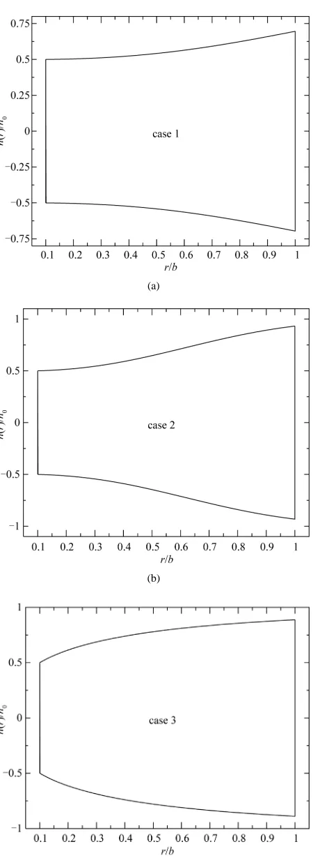
For both disks, h0 is the thickness at the inner edge of the disk, n and k are geometric parameters, a is the inner radius of the disk and b is the outer radius of the disk (see Figures 1 and 2). The value of n equal to zero represents a uniform-thickness annular disk. It is to be noted that the parameter n determines the thickness at the outer edge of the annular disk relative to h0 while the parameter k determine the shape of the profile. The thickness of the annular disk 1 may be decreases at the outer edge (see Figure 1) while the thickness of the an-nular disk 2 may be increases at the outer edge (see Fig-ure 2). The value of k equal to unity represents a linearly decreasing variable thickness for the annular disk 1 while it represents a linearly increasing variable thickness for the annular disk 2. The geometric parameters k and n are given according to three cases. In case 1: k = 2.5, n = 2, in case 2: k = 2.5, n = 0.5, and in case 3: k = 0.6, n = 2.
(a)
(b)
[image:3.595.56.287.62.691.2](c)
Figure 1. Variable-thickness annular disk 1 profiles for (a) case 1, (b) case 2 and (c) case 3.
(a)
(b)
(c)
[image:3.595.313.538.67.687.2]
1 2
2 2
0
1 1
, , r, .
r
bh
Then, Equation (7) may be written in the following simple forms according to the two cases:
2 2 2 3 d d 1 d d1 e 0,
k k
k
n R A k
R knR R
R R
kn R R
(11)
for annular disk 1, and
2 2 2 3d e d
1
d
d 2 e
e
1 2 e 0,
2 e k k k k k k k k k k
n R A k
n R A n R A k
n R A n R A
knR R R R R kn R R (12)
for annular disk 2.
3. Exact and Numerical Solutions
The exact general solution for Equation (11) may be available while it is not available for Equation (12). The modified Runge-Kutta numerical solution may be avail-
The exact general solution for Equation (11) can be written as
1 1
2 2
1 , 2 ,
e nRk k enAk
i j i j
R R c W R c M R P R
,
(13)
where c1 and c2 are arbitrary constants and Wi j,
Rand Mi j,
R are Whittaker’s functions (seeAbramo-witz and Stegun [16]),
, , , , , , , ,
i j i j
M R M i j z W R W i j z (14)
in which 2 1 , , . 2 k k
i j z nR
k k
(15)
It is to be noted that Whittaker’s functions may be given by
1 1 2 2 1 1 2 2 1, , e , 1 2 , ,
2
1
, , e ,1 2 , ,
2
z j
z j
M i j z z H j i j z
W i j z z K j i j z
(16)
where H and K are the hypergeometric and Kummer’s functions, respectively, with n > 0. It is to be noted that for real values of i and j, Whittaker’s functions Wi j,
Rand Mi j,
R converge for 1k
R .
The termP R
in Equation (13) can be written as
j
j
d j
j d ,P R W R
P R M R RM R
P R W R R (17) where
1 1
2 2 2
, 1, 1, ,
e
.
1 ( )
k
nR k
i j i j i j i j
R P R
kM R W R M R W R
(18)
The substitution of Equation (13) into Equation (5) with the aid of the dimensionless forms given in
Equa-tion (10) gives the radial and circumferential stresses in the following forms:
1 1
2 2 1
1 1 , 2 ,
2 2
e e ,
d
e .
d 3
k k
k k
nR k nA
i j i j
n R A
R R c W R c M R P R
R R R R (19)
Note that the first differentiations of Whittaker’s func- tions Wi j,
R and Mi j,
R are given by
, , 1,
, , 1,
d 1
,
d 2
d 1 1
.
d 2 2
k
i j i j i j
k
i j i j i j
k
W R nR i W R W R
R R
k
M R nR i M R i j M R
Finally, the dimensionless strains and the correspond- ing radial displacement may be obtained easily using Equation (19) as well as the dimensionless forms given in Equation (10). So, all of stress function, stresses, strains, and radial displacement can be completely de-termined under the traction conditions on the inner and outer surfaces of the annular disk. They can be expressed as
0 0 at ,
0 0 at 1 .
r a R A
r b R
(21)
3.2. Numerical Solution
The modified Runge-Kutta algorithm may be used here to solve both the differential Equations (11) and (12) with the aid of the boundary conditions given in Equa- tion (21). Equations (11) or (12) can be written in the following general form:
, , , 1, 2.
s s s
s
f R s
(22)
where the prime denotes differentiation with respect to R and s denotes the disk number. The functions fs may
be given by
1 1
1 2
1 1
e ,
k k
k k
n R A
knR kn R
f R
R R
(23)
2 2 2 2 1 e 1 2 e 1 e 1 2 e2 e .
k k
k k
k k
k k
k k
n R A k
n R A n R A k
n R A n R A
knR f R kn R R R (24)
Runge-Kutta’s iterative formulae for the second-order differential equation are [11-14]
1 1 2 3 4
1 1 2 3
2 2 ,
6
, 6
s s s s s s
i i
s s s s s s
i i i
R
K K K K
R
R K K K
(25)
where R is the increment of the distance along the radial direction of the rotating annular disks, and
, 1, 2, 3, 4
s j
K j can be determined with the following relations
1 2 1 23 1 2
2
4 2 3
, , ,
1 1 1
, , ,
2 2 2
1 1 1 1
, , ,
2 2 4 2
1
, , .
2 i
s s s
s i i i
s
s s s s
s i i i
s s s s s s
s i i i i
s s s s s s
s i i i i
K f R
K f R R R RK
K f R R R R K RK
K f R R R R K RK
(26)
The numerical simulation starts from the inner boun-dary, where a trial value of the first derivative of the stress function is assumed. With a small distance R, the stress function and its first derivative at the new posi-tion can be obtained using Equaposi-tion (25) and the radial stress is calculated. According to the difference between the computed radial stress and the known radial stress at the outer boundary, the initial trial value of the first de-rivative of the stress function at the inner boundary is modified and the next iteration is carried out in the same way. This iterative process is performed until both the boundary conditions are simultaneously satisfied. Once the stress function is obtained, the stresses, strains, and displacement in the rotating annular disks can be ob-tained using Equations (2), (5) and (6) with the aid of the dimensionless given in Equation (10). This process may be easily done after getting the continuous form of the stress function using the curve fitting and least square
method. So, all other quantities can be easily determined.
4. Numerical Examples and Discussion
Some numerical examples for the rotating variable- thickness annular disk will be given according the exact and numerical solutions ( 0.3). Results determined as per the exact analytical solution are compared with those obtained by the numerical Runge-Kutta (R-K) so-lution in Figures 3-10 for disk 1. Additional results for stress function, radial displacement, strains and stresses of the rotating variable-thickness annular disk 2 using the numerical R-K solution are also presented in Figures 11-16. The inner and outer radii of the disk are taken to be a = 0.1 b (R = A = 0.1) and b (R = 1), and the results are given in terms of the rotating angular velocity.
Figure 3. Stress function Ф, radial stress σ1 and circumfer-
[image:6.595.58.290.74.254.2]ential stress σ2 in the variable-thickness annular disk 1.
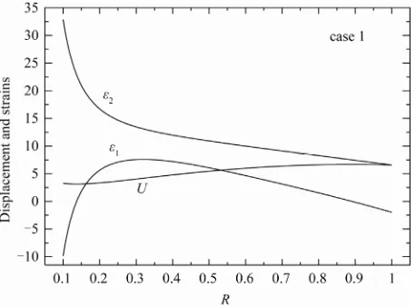
Figure 4. Displacement U, radial strain ε1 and circumferen-
tial strain ε2 in the variable-thickness annular disk 1.
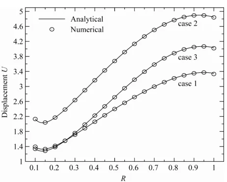
[image:6.595.309.536.292.470.2]Figure 5. Displacement U of the variable-thickness annular disk 1 for all cases.
Figure 6. Stress function Ф of the variable-thickness annu- lar disk 1 for all cases.
Figure 7. Radial stress σ1 in the variable-thickness annular
disk 1 for all cases.
Figure 8. Circumferential stress σ2 in the variable-thickness
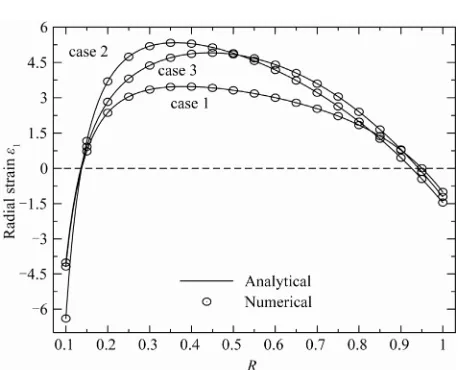
[image:6.595.57.288.295.473.2] [image:6.595.56.287.506.691.2] [image:6.595.309.538.513.689.2]Figure 9. Radial strain ε1 in the variable-thickness annular
[image:7.595.56.288.294.470.2]disk 1 for all cases.
Figure 10. Circumferential strain ε2 in the variable-thick-
ness annular disk 1 for all cases.
that being reported herein, with help of Equation (10), are in the following dimensionless forms:
U, 1, 2, , 1, 2
100
U, 1, 2, , 1, 2
. (27) The distribution of the stress function and stresses are presented in Figure 3 while the distribution of the radial displacement and strains are presented in Figure 4. The results are given for rotating variable-thickness annular disk with k = 2.5 and n = 2 (case 1). The numerical R-K solution is compared with the exact analytical solution. It is clear that, R-K method gives all results with excellent accuracy when compared with the exact analytical solu-tion.The distributions of the stress functions, radial stress, circumferential stress, radial displacement, radial strain as well as circumferential strain through the radial direc-tion of the annular disk 1 are all presented in Figures
5-10, respectively, for different cases of the geometric parameters k and n. Figure 5 shows that the radial dis-placement U has minimum value near the inner edge (at R = 0.15) and maximum value near the outer edge (at R = 0.9) for all cases of the parameters k and n. Cases 1 and 3 (n = 2) are coincided with each other when R = 0.2. Case 2 with small n (n = 0.5) gives the highest values of the displacement.
Figure 6 shows that the stress function has its maximum at the mid-plane of the disk (R = 0.55) for case 2 while its maximum occurs at (R = 0.45) and (R = 0.5) for cases 1 and 3, respectively. Once again, cases 1 and 3 are coincided with each other when R = 0.7. Case 2 with small n gives the highest values of the stress function.
The radial stress 1 and circumferential stress 2 in the rotating variable-thickness annular disk 1 are plot-ted in Figures 7 and 8. The maximum value of 1 does not occur at the mid-plane of the disk 1. It occurs at R = 0.33, R = 0.43, R = 0.35 for cases 2, 3 and 1, respectively. The maximum value of 2 occurs at the inner surface of the disk 1 while the smallest value occurs at outer surface. Case 1 gives the smallest stresses. The same conclusion may be applied on the plots of strains in Fig-ures 9 and 10.
It can be seen from Figures 3-10 that the R-K method can describe all results through-the-thickness of the ro-tating annular disk 1 very well enough. This puts into evidence the great role played by R-K method in the modeling of rotating variable-thickness annular disks. So, it will trustily used to find the solution for Equation (12) of the rotating variable-thickness annular disk 2. As a result, the stresses and stress function in the rotating va-riable-thickness disk 2 are plotted in Figures 11-13 ac-cording to all cases. However, the radial displacement and strains are plotted in Figures 14-16.
Figure 11. Stress function Ф, radial stress σ1 and circum-
ferential stress σ2 in the variable-thickness annular disk 2
[image:7.595.308.537.509.681.2]Figure 12. Stress function Ф, radial stress σ1 and circum-
ferential stress σ2 in the variable-thickness annular disk 2
for case 2.
Figure 13. Stress function Ф, radial stress σ1 and circum-
ferential stress σ2 in the variable-thickness annular disk 2
[image:8.595.59.289.75.245.2]for case 3.
Figure 14. Displacement U, radial strain ε1 and circumfer-
ential strain ε2 in the variable-thickness annular disk 2 for
[image:8.595.57.287.291.465.2]case 1.
Figure 15. Displacement U, radial strain ε1 and circumfer-
ential strain ε2 in the variable-thickness annular disk 2 for
[image:8.595.308.536.294.466.2]case 2.
Figure 16. Displacement U, radial strain ε1 and circumfer-
ential strain ε2 in the variable-thickness annular disk 2 for
case 3.
5. Conclusions
[image:8.595.58.287.514.683.2]were compared. The proposed R-K approach gives very agreeable results to the exact analytical solution. The modified R-K method presented here may be trustily used for the boundary value problems that their exact solutions are not available.
6. References
[1] S. P. Timoshenko and J. N. Goodier, “Theory of Elastici-ty”, McGraw-Hill, New York, 1970.
[2] S. C. Ugral and S.K. Fenster, “Advanced Strength and Ap- plied Elasticity”, Elsevier, New York, 1987.
[3] U. Güven, “Elastic-Plastic Stresses in a Rotating Annular Disk of Variable Thickness and Variable Density,” In-ternational Journal of Mechanical Sciences, Vol. 34, 1992, pp. 133-138.
[4] U. Güven, “On the Stress in the Elastic-Plastic Annular Disk of Variable Thickness under External Pressure,” In-ternational Journal of Solids and Structures, Vol. 30, 1993, pp. 651-658.
[5] U. Güven, “Stress Distribution in a Linear Hardening Annular Disk of Variable Thickness Subjected to Exter-nal Pressure,” International Journal of Mechanical Sci- ences, Vol. 40, 1998, pp. 589-601.
doi:10.1016/S0020-7403(97)00081-7
[6] A. M. Zenkour, “Analytical Solutions for Rotating Ex-ponentially-Graded Annular Disks with Various Boun-dary Conditions,” International Journal of Structural Stability and Dynamics, Vol. 5, 2005, pp. 557-577.
doi:10.1142/S0219455405001726
[7] A. M. Zenkour and M. N. M. Allam, “On the Rotating Fiber-Reinforced Viscoelastic Composite Solid and An-nular Disks of Variable Thickness,” International Journal for Computational Methods in Engineering Science & Mechanics, Vol. 7, 2006, pp. 21-31.
doi:10.1080/155022891009639
[8] A. M. Zenkour, “Thermoelastic Solutions for Annular Disks with Arbitrary Variable Thickness,” Structural En-gineering and Mechanics, Vol. 24, 2006, pp. 515-528. [9] O. C. Zienkiewicz, “The Finite Element Method in
Engi-neering Science,” McGraw-Hill, London, 1971.
[10] P. K. Banerjee and R. Butterfield, “Boundary Element Methods in Engineering Science,” McGraw-Hill, New York, 1981.
[11] M. L. James, G. M. Smith and J. C. Wolford, “Applied Numerical Methods for Digital Computation,” Harper & Row, New York, 1985
[12] L. H. You, Y. Y. Tang, J. J. Zhang and C.Y. Zheng, “Numerical Analysis of Elastic-Plastic Rotating Disks with Arbitrary Variable Thickness and Density,” Interna-tional Journal of Solids and Structures, Vol. 37, 2000, pp. 7809-7820. doi:10.1016/S0020-7683(99)00308-X
[13] C. F. Gerald and P. O. Wheatley, “Applied Numerical Analysis,” 6th Edition, Addison-Wesley, California, 2002.
[14] M. H. Hojjati and A. Hassani, “Theoretical and Numeri-cal Analysis of Rotating Discs of Non-Uniform Thick-ness and Density,” International Journal of Pressure Vessels and Piping, Vol. 85, 2008, pp. 694-700.
doi:10.1016/j.ijpvp.2008.02.010
[15] M. H. Hojjati and S. Jafari, “Semi-Exact Solution of Elastic Non-Uniform Thickness and Density Rotating Disks by Homotopy Perturbation and Adomian’s De-composition Methods. Part I: Elastic Solution,” Interna-tional Journal of Pressure Vessels and Piping, Vol. 85, 2008, pp. 871-878. doi:10.1016/j.ijpvp.2008.06.001